Overview

In this project, We aimed to investigate the relationship between the influence of unobserved confounders and the deviation of spurious correlation from the true causal effect. This is similar to the concept of sensitivity analysis in the causal effect estimation. We utilized entropy as a measure to quantify the strength of the confounder and developed an algorithm to estimate bounds for the causal effect based on the observational distribution and the strength of confounders.

Checkout Our Paper and Codes

Approximate Causal Effect Identification under Weak Confounding[arXiv][code][video] Published in International Conference on Machine Learning (ICML), 2023

Quantify the Confounder’s Strength

Many studies use information theoretic quantities to measure the strength of edges in the causal graph, such as Entropic Causal Inference (Kocaoglu et al. 2017) and causal strength (Janzing et al. 2012). Inspired by these works, we consider the mutual information $I(X;Z)$ and $I(Y;Z)$ as the information between $X$ and $Y$ through the backdoor channel $Z$. Since $I(X;Z), I(Y;Z)\leq H(Z)$, we use entropy to quantify the strength of confounders.

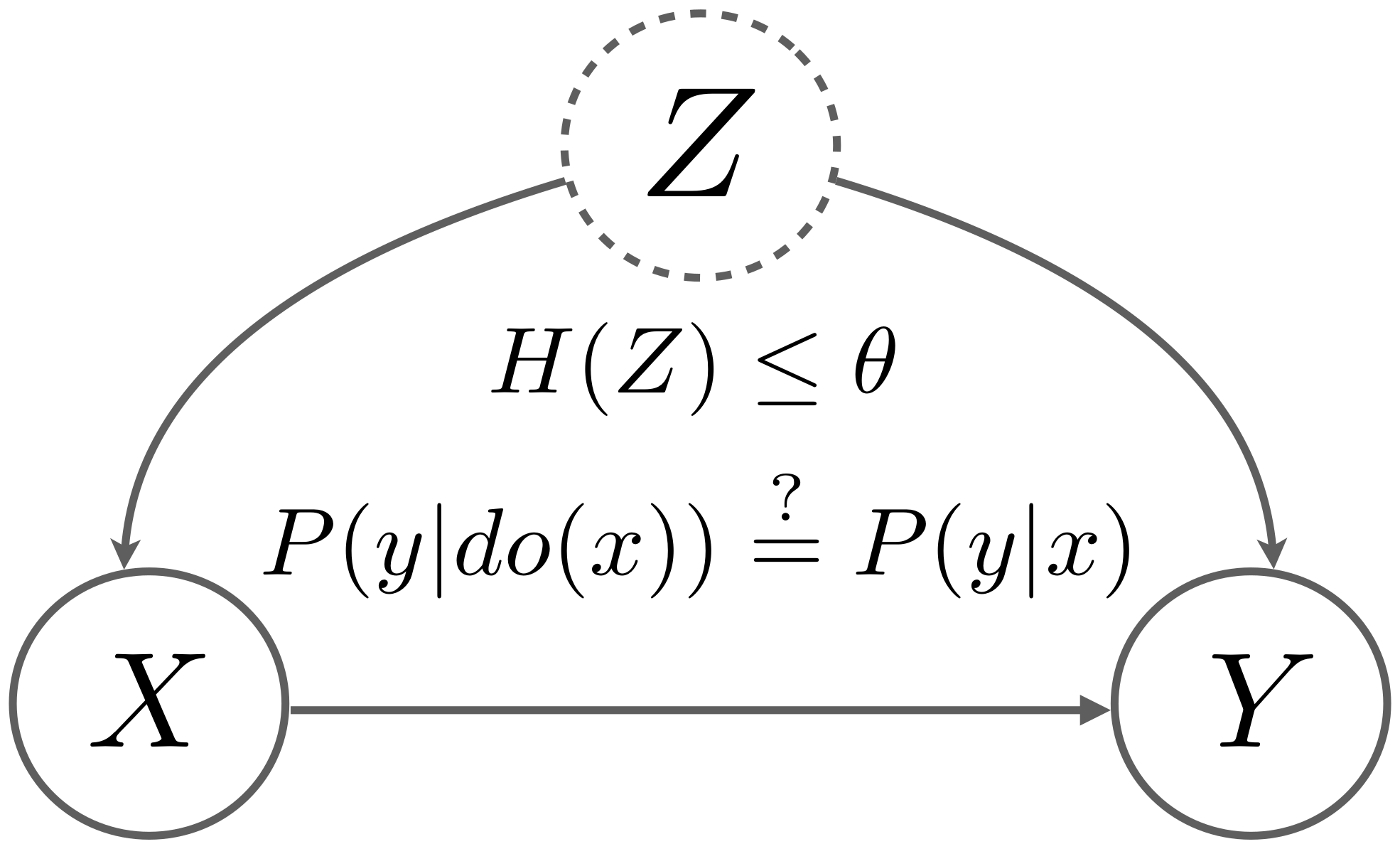
We want to draw connections between the strength of confounders and the deviation of causal effect due to the backdoor path. Formally, the problem is defined as:

$$ \text{Given }P(X, Y )\text{ and } H(Z)\leq θ,\text{ finding the }\min / \max P(y | do(x)). $$

The Canonical Partition Method

One can use the backdoor adjustment to estimate the causal effect if the confounder is observed. However, this method is not suitable for this problem. Due to the concavity of the entropy function, imposing the entropy constraint on the optimization problem results in a non-convex feasible set.

The Canonical Partition is a commonly used method for studying causal effects. It involves discrete variables $X$ and $Y$, and introduces variables $R_x$ and $R_y$ to represent the various possible mappings from $X$ to $Y$. Essentially, these response variables serve as parameters that capture the randomness of the functions responsible for mapping $X$ to $Y$.

When $X$ and $Y$ are binary variables, there are four possible mechanisms that depict how variable $Y$ responds to variable $X$, as illustrated in the figure below.

Since $X$ is an exogenous variable given the observational distribution, we have $P(R_x) = P(X)$. As a result, we can use a total of 8 states to represent $P(R_x, R_y)$. We can represent the causal effect and observational distribution with the joint distribution of response variables $P(R_x, R_y)$.

$$ P(y|do(x)) = \sum_{i=0}^{1} \sum_{j=0}^{1} P(R_y=i, R_x=j) $$ $$ P(x,y) = P(R_y=0, R_x=0)+ P(R_y=1, R_x=0) $$ $$ P(x,y) = P(R_y=2, R_x=0)+ P(R_y=3, R_x=0) $$

From the above equation, Tian and Pearl (2000) showed the causal effect can be bounded as

$$ P(x,y) \leq P(y|do(x)) \leq 1- P(x,y′). $$

To apply the entropy constraint, observe that the $R_x$ and $R_y$ are conditionally independent given the confounder $Z$.

By the data processing inequality, the mutual information $I(R_x;R_y)$ is bounded by the entropy of $Z$. And since mutual information is a convex function of the conditional distributions $P(R_y|R_x)$, we can form the optimization problem as below.

Given $P(X,Y)$ for $ |X|=n, |Y|=m$ and entropy constraint $H(Z)\leq \theta$. The upper and lower bounds of causal effect $P(y_p|do(x_q))$ is given by

Here $a_{ij}$ are the optimization parameters correspond to $P(R_y=i|R_x=j)$.

Since the variable $R_y$ represents all possible mapping from $X$ to $Y$, we have the number of states $|R_y|=m^n$, and total number of parameters $|a|=nm^n$. The number of parameters grow exponentially with the number of states of $X$. So the optimization may become intractable for $X, Y$ in high dimensions.

To encounter this issue, we utilize a different parameterization of causal effect.

The Single World Intervention Graphs

The Single World Intervention Graph (SWIG) is a graphical representation to link the counterfactual distribution and DAG introduced by Richardson and Robins (2013).

Here $Y_x$ denotes the distribution of $Y$ after the intervention $do(X=x)$. By the graphical independency condition (also by the ignorability assumption), we have $Y_x$ and $X$ are conditionally independent given $Z$.

Again, by the data processing inequality, the mutual information $I(Y_x;X)$ is bounded by the entropy of confounder $H(Z)$. And we can formulate the optimization problem with the counterfactual distribution $P(Y_x, X)$ as below.

Given $P(X,Y)$ for $ |X|=n, |Y|=m$ and entropy constraint $H(Z)\leq \theta$. The upper and lower bounds of causal effect $P(y_p|do(x_q))$ is given by

Here $b_{ij}$ are the optimization parameters correspond to $P(Y_x=i|X=j)$. We have $|Y_x|=m$ and $|b|=mn$.

The Entropy Threshold

Now we want to determine the threshold of the entropy constraint such that its application yields tighter bounds. First, we look at the optimization parameters $b_{ij}$ in the conditional probability table.

The causal effect achieves Tian-Pearl upper/lower bounds when the red row is maximized/minimized.

First, we demonstrate that for binary variables $X$ and $Y$, maximizing the mutual information $I(Y_x;X)$ results in the achievement of bounds for a certain instance of causal effect. Assume, without loss of generality, $P(y|x) ≥ P(y′|x)$. The threshold of entropy constraint for obtaining tighter bounds is shown in the figure below.

The brightness of the plot represents the gap between upper and lower bounds when the entropy constraint equals the threshold. So without the entropy constraint, the gap between upper and lower bounds is monotonically decreasing with $P(x)$.

Next, we present several lemmas to determine the entropy threshold for non-binary $X$ or $Y$. In particular, we demonstrate that when either $X$ or $Y$ is binary, we can transform the optimization problem into the binary case by constructing a distribution $P(U,V)$. Consequently, we can extend the intuition from the binary $X,Y$ scenario to situations where either $X$ or $Y$ is non-binary.

The following figure shows the gap of our bounds vanishes as the entropy converge to zero. Each subplot represents a distribution of $P(X,Y)$. The green curves are the bounds given the entropy constraint and the red curves are the Tian-Pearl bounds.

Experiments

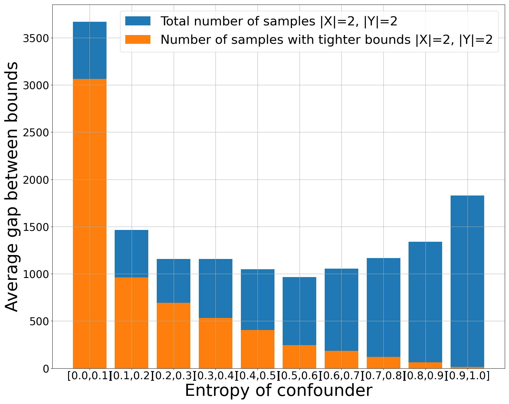
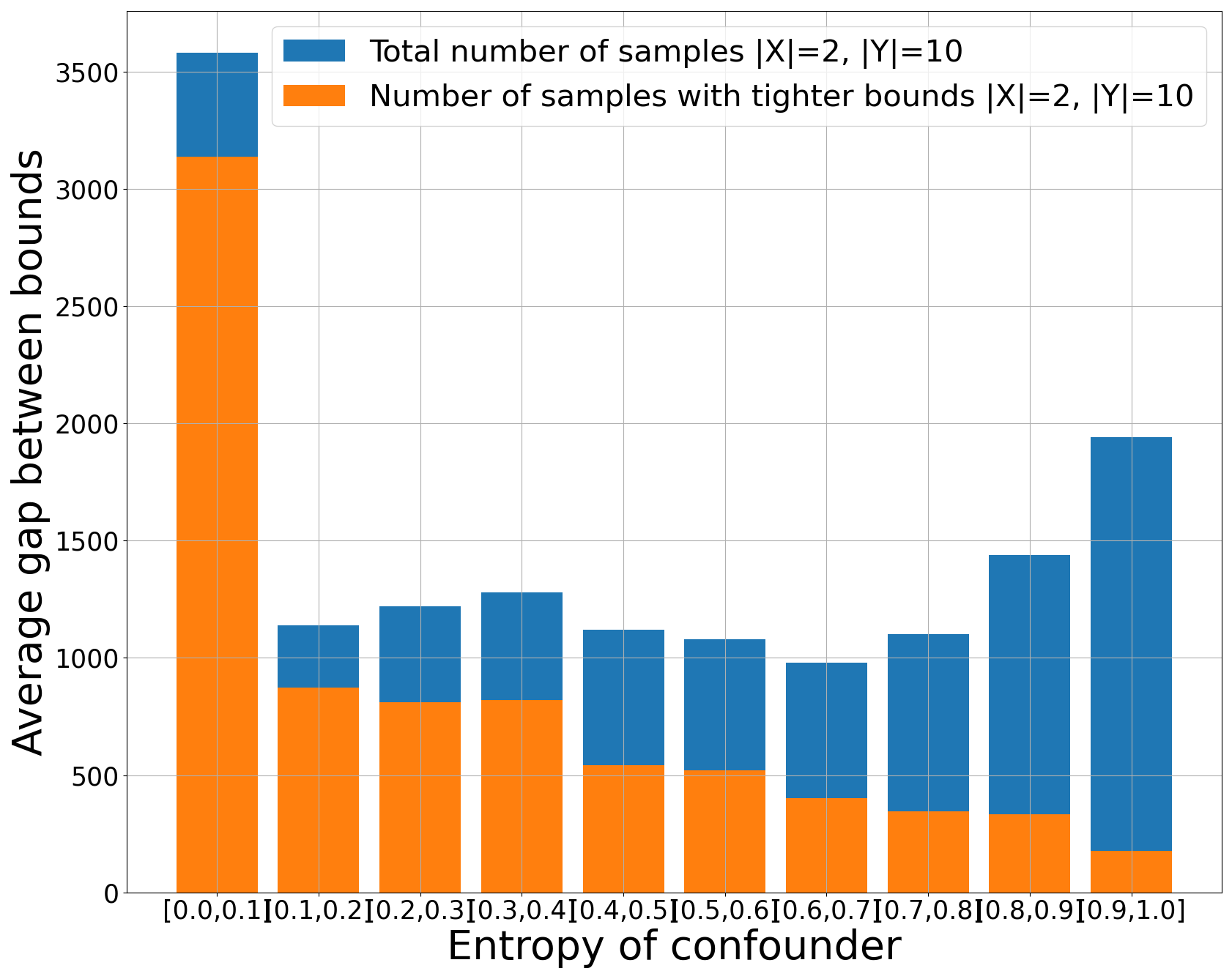
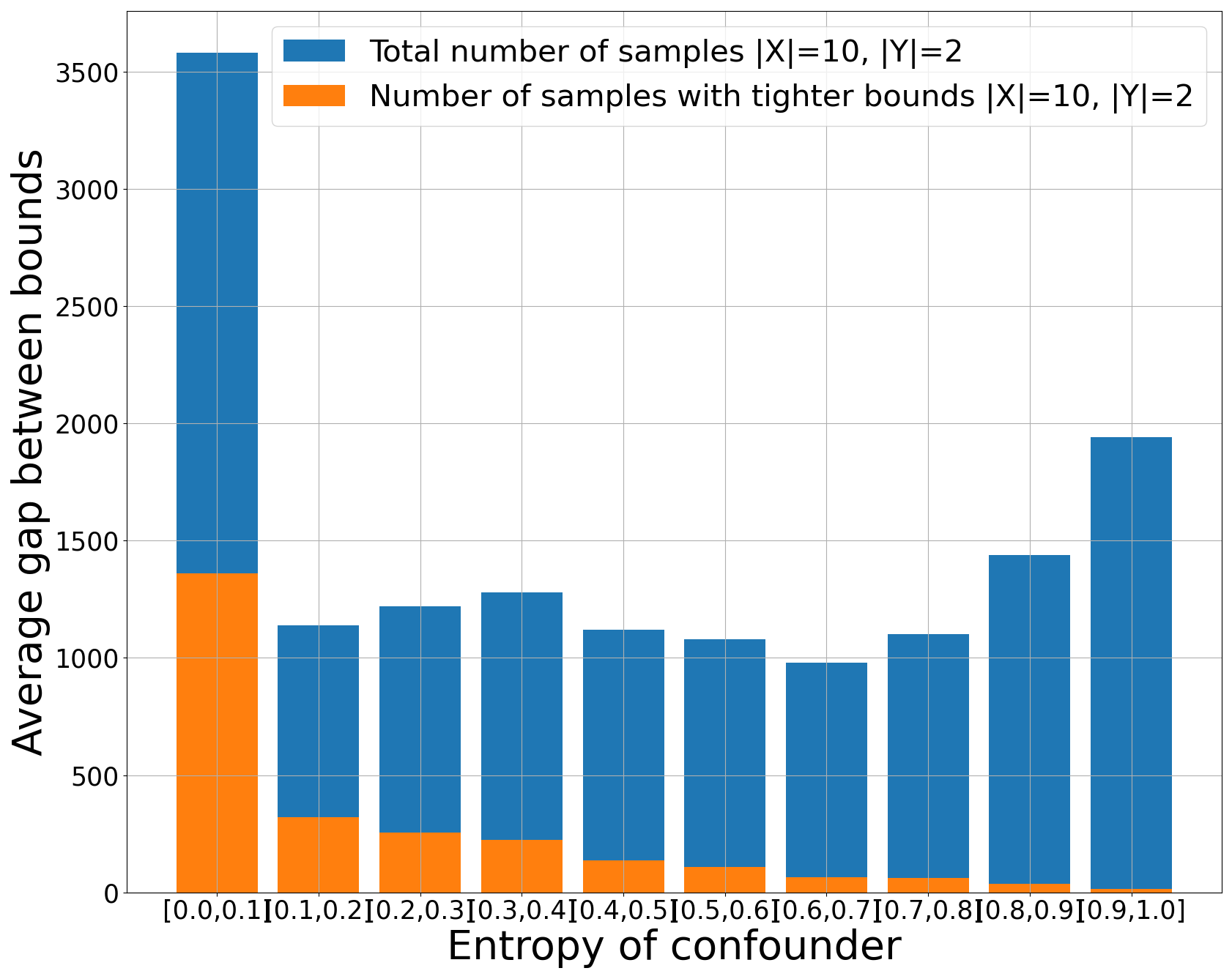
We conducted experiments using both simulated and real-world data. For the simulated data, we generated distributions based on the given graph, incorporating small entropy confounders. Using the joint distribution $P(X, Y)$ and $H(Z)$, we computed the bounds of the causal effect. The figure below illustrates the average gap between bounds, grouped by entropy.

The number of samples that yield tighter bounds is shown in the figures below.

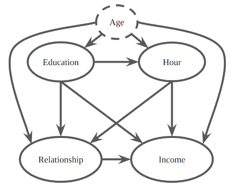
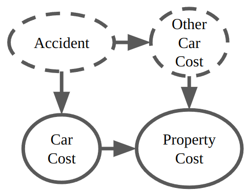
Regarding the real-world dataset, we selected a subset of variables and assumed that the confounders were not jointly observed; only the prior distributions were available. We demonstrated that our methods produced tight bounds even in the presence of small entropy confounders. These findings offer valuable information and guidance for decision-making processes.

For more details about the experiments, please refer to our paper.

BibTeX

@InProceedings{jiang2023approximate,
  title={Approximate Causal Effect Identification under Weak Confounding},
  author={Jiang, Ziwei and Wei, Lai and Kocaoglu, Murat},
  booktitle={International Conference on Machine Learning},
  pages={15125--15143},
  year={2023},
  organization={PMLR}
}