Here are the assignments for the Robotics Specialization: Aerial Robotics offered by UPenn on Coursera.

In this course, we learned some basic ideas about autonomous robots and the design of quadrotors. There are three assignments in this course in which we learned to design a PD controller for a quadrotor in 1D, 2D, and 3D. The course provided quadrotor simulators to help with the experiment. The simulator uses MATLAB’s ODE solver, ode45, to simulate the behavior of the quadrotor and plt3 to visualize the state of the quadrotor at each time step.

1D Quadrotor Control

For the first part, we only consider the motion in $z$-axis as shown in the figure.

The net force in the vertical direction is given by $$F=m\ddot{z} = u - mg$$ where $u$ is the rotor thrusts. The dynamic of the quadrotor in the vertical direction can be described by the following differential equation $$\ddot{z}= \frac{u}{m}- g.$$

We can measure the current position and velocity of the quadrotor in the vertical direction. Then we can use these and desired position and velocity to calculate the errors $$e = z_{des} - z.$$

The control input for a PD controller is $$u=m(\ddot{z}+ K_pe + K_d\dot{e} +g)$$ By choosing proper values for proportional and derivative gain, we can make the quadrotor respond quickly to a step input. The result is as

2D Quadrotor Control

For the second part, we learned to control the quadrotor in the 2D plane, as shown in the following figure.

In the figure, $a_2, a_3$ denote the inertial frame, and $b_2, b_3$ denote the body frame. In this setup, we want to control the quadrotor’s elevation and roll angle with two inputs: the thrust force ($u_1$) and the moment ($u_2$). The thrust force is defined as the sum of the thrusts at each rotor $$u_1 = F_1+F_2,$$ and the moment is the difference between the thrusts of two rotors times the arm length of the quadrotor ($L$), $$u_2 = L(F_1 - F_2).$$

Suppose we can measure the position, velocity, acceleration, and angular acceleration of the robot. Let $r=[y, z]^T$ denote the position vector of the quadrotor in the inertial frame, and $R$ be the rotation matrix that transforms vector components from the body frame to the inertial frame. $$ R = \begin{bmatrix} \cos(\phi) & -\sin(\phi) \\ \sin(\phi) & \cos(\phi) \end{bmatrix} $$ The net force in the $Y, Z$ direction is given by $$ m \begin{bmatrix} \ddot{y} \\ \ddot{z} \end{bmatrix} = \begin{bmatrix} 0 \\ -mg \end{bmatrix} + R\begin{bmatrix} 0 \\ u_1 \end{bmatrix} = \begin{bmatrix} 0 \\ -mg \end{bmatrix} + \begin{bmatrix} -u_1 \sin(\phi) \\ u_1\cos(\phi)\end{bmatrix}.$$ The angular acceleration is given by $$ I_{xx}\ddot{\phi} = L(F_1 - F_2) = u_2.$$ Therefore, the system model is given by $$\begin{bmatrix} \ddot{y} \\ \ddot{z} \\ \ddot{\phi} \end{bmatrix} = \begin{bmatrix} 0 \\ -g \\ 0 \end{bmatrix} + \begin{bmatrix} -\frac{1}{m} \sin(\phi) & 0 \\ \frac{1}{m} \cos(\phi) & 0 \\ 0 & \frac{1}{I_{xx}}\end{bmatrix} \begin{bmatrix} u_1 \\ u_2\end{bmatrix}.$$

The dynamic model of the quadrotor is nonlinear, so we need to linearize the equation of motions in order to apply the PD controller. For the quadrotor, the equilibrium point is the configuration at any position $(y^{(t)}, z^{(t)})$ with zero roll angle; and the thrust force is equal to the gravity $mg$. So we have $y^{(t)}, z^{(t)}, \phi^{(t)}=0, u_1^{(t)} = mg, u_2^{(t)} = 0$. By the first-order Taylor approximation, we have $\sin(\phi^{(t)})\approx 0, \cos(\phi^{(t)}) \approx 1$. Thus the above system model can be written as $$\begin{bmatrix} \ddot{y} \\ \ddot{z} \\ \ddot{\phi} \end{bmatrix} = \begin{bmatrix} -g\phi \\ -g + \frac{u_1}{m} \\ \frac{u_2}{I_{xx}} \end{bmatrix}, $$ and $$ \begin{bmatrix} u_1 \\ u_2 \\ \phi \end{bmatrix} = \begin{bmatrix} m(\ddot{z} +g) \\ I_{xx}\ddot{\phi} \\ -\frac{\ddot{y}}{g} \end{bmatrix}. $$

Let $s$ denotes the state variable $(y$, $z$ or $\phi)$ and $s_T(t)$ be the desired state variable at time $t$. Define the position and velocity errors as $$\begin{bmatrix} e \\ \dot{e} \end{bmatrix} = \begin{bmatrix} s_T(t) - s \\ \dot s_T(t) - \dot{s}\end{bmatrix}.$$ The error should satisfy the following differential equation, $$ (\ddot r_T(t) - \ddot{r}) + K_d\dot{e} + K_pe = 0. $$ So the commanded acceleration of the state can be expressed as $$ \ddot{r} = \ddot r_T(t) + K_d\dot{e}+ K_pe . $$ The input can be expressed as $$ \begin{bmatrix} u_1 \\ u_2 \\ \phi \end{bmatrix} = \begin{bmatrix} m(\ddot z_T(t) + K_{d,z}(\dot z_T(t)-\dot z)+ K_{p,z}(z_T(t) - z) +g) \\ I_{xx}(\ddot \phi_T(t) + K_{d,\phi}(\dot \phi_T(t)-\dot \phi)+ K_{p,\phi}(\phi_T(t) - \phi)) \\ -\frac{1}{g} (\ddot y_T(t) + K_{d,y}(\dot y_T(t)-\dot y)+ K_{p,y}(y_T(t) - y))\end{bmatrix} .$$ The resulting controller is shown below.

3D Quadrotor Control

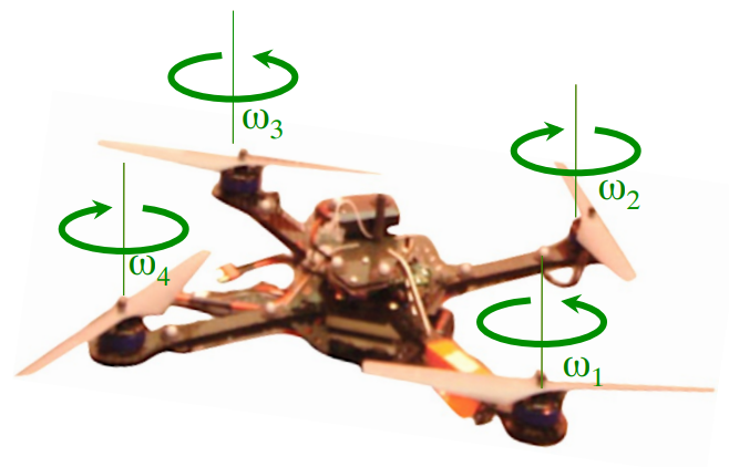
The last part of this course involves controlling the quadrotor in the 3D world coordinates. To represent the state of the quadrotor, we use rotation matrix $Z-X-Y$ with the axis of the world frame. The coordinate system is shown in the figure below, where $\mathbf{a_i}$ represents the world frame, and $\mathbf{b_i}$ represents the body frame.

The rotation matrix for transform from $\mathcal{A}$ to $\mathcal{B}$ can be represented by the yaw angle $\psi$, roll angle $\phi$, and pitch angle $\theta$:

$$ ^\mathcal{A}[R]_\mathcal{B} = \begin{bmatrix} \cos\psi\cos\theta-\sin\phi\sin\psi\sin\theta & -\cos\phi\sin\psi & \cos\psi\sin\theta + \cos\theta\sin\phi\sin\psi \\ \cos\theta\sin\psi + \cos\psi\sin\phi\sin\theta & \cos\phi\cos\psi & \sin\psi \sin\theta - \cos\psi\cos\theta\sin\phi \\ -\cos\phi\sin\theta & \sin\phi & \cos\phi\cos\theta \end{bmatrix}.$$

The angular velocity of the quadrotor in the body frame $\mathcal{B}$ can be represented by: $$^\mathcal{A}\omega_\mathcal{B} = p\mathbf{b_1} + q\mathbf{b_2} + r\mathbf{b_3},$$ where $p, q,$ and $r$ are related to the roll, pitch, and yaw angles as $$ \begin{bmatrix} p\\ q\\ r\\ \end{bmatrix} = \begin{bmatrix} \cos\theta & 0 &-\cos\phi\sin\theta \\ 0 & 1 & \sin\phi \\ \sin\theta & 0 & \cos\phi\cos\theta \end{bmatrix}\begin{bmatrix} \dot{\phi} \\ \dot{\theta} \\ \dot{\psi} \end{bmatrix}.$$

Next we express the thrust force $F_i$ and moment $M_i$ that produced by each rotor with the angular speed $\omega_i$, $$ F_i = k_F\omega_i^2,$$ and $$ M_i = k_M\omega_i^2.$$ The constant $k_F \approx6.11 \times 10^{-8} \frac{N}{rpm^2}$, and $k_M \approx 1.5\times 10^{-9} \frac{Nm}{rpm^2}$.

Then we can relate the force produced by rotors with the quadrotor motion with Newton’s equation of motion

$$m\mathbf{\ddot{r}} = \begin{bmatrix} 0 \\ 0\\ -mg\end{bmatrix} + \mathbf{R} \begin{bmatrix} 0\\ 0 \\ \sum_{i=1}^4 F_i \end{bmatrix}.$$

From Euler’s equation of motion, we can relate the angular acceleration with the thrust force. Since the moment produced by each rotor is in the reverse direction of its rotation, the moment from the rotor 1 and 3 are in $\mathbf{b_3}$ direction; the rotors 2 and 4 produce moment in $-\mathbf{b_3}$ direction. Then by the Euler equation, we have

$$ I\begin{bmatrix} \dot{p} \\ \dot{q} \\ \dot{r} \end{bmatrix} = \begin{bmatrix} L(F_2-F_4) \\ L(F_3-F_1) \\ M_1 -M_2+M3 -M_4 \end{bmatrix} - \begin{bmatrix} p\\ q\\ r\end{bmatrix} \times I \begin{bmatrix} p \\ q \\ r \end{bmatrix},$$ where $L$ is the distance from the rotor to the center of mass. Let $\gamma = \frac{k_M}{k_F}$, the above equation can be rewrite as $$ I\begin{bmatrix} \dot{p} \\ \dot{q} \\ \dot{r} \end{bmatrix} = \begin{bmatrix} 0 & L &0 &-L \\ -L & 0 & L & 0 \\ \gamma & -\gamma & \gamma & -\gamma \end{bmatrix} \begin{bmatrix} F_1 \\ F_2 \\ F_3 \\ F_4 \end{bmatrix} - \begin{bmatrix} p \\ q \\ r \end{bmatrix} \times I \begin{bmatrix} p \\ q \\ r \end{bmatrix}$$

In this project, we consider two sets of input, the net thrust force $u_1 = \sum_{i=1}^4 F_i $ and a vector $\mathbf{u_2} = \begin{bmatrix} L(F_2-F_4) \\ L(F_3-F_1) \\ M_1 - M_2 +M_3 -M_4 \end{bmatrix}$, a function of thrust and moment. The controller is designed to perform hovering or trajectory following.

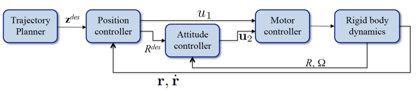
As shown in the figure above, the outer loop controls the position from the error in the position vector and desired position. The inner loop controls the attitude of the quadrotor with the onboard accelerometers and gyros. The desired trajectory is represented by $$ \mathbf{z}_{des} = \begin{bmatrix} \mathbf{r}_T(t) \\ \psi_T(t) \end{bmatrix}. $$

The PD controller for attitude control is $$ \mathbf{u_2} = \begin{bmatrix} k_{p,\phi}(\phi_{des} - \phi)+ k_{d,\phi}(p_{des}-p) \\ k_{q,\theta} (\theta_{des} - \theta) + k_{d,\theta}(q_{des} - q) \\ k_{r,\phi}(\psi_{des} - \psi) + k_{d, psi}(r_{des}-r) \end{bmatrix} $$

Similar to the 2D case, we linearize the equation of motions to apply the PD controller. The equilibrium point is the configuration at the position where the angular velocity is equal to zero; the pitch and roll angle are close to zero.

Linearizing Newton’s equation, get $$ \ddot{r_1} = g(\Delta \theta \cos\psi_0 + \Delta\phi\sin\psi_0)$$ $$ \ddot{r_2} = g(\Delta \theta \sin\psi_0 - \Delta\phi\cos\psi_0)$$ $$\ddot{r_3} = \frac{1}{m}u_1 - g.$$

Linearizing Euler’s equation, get

$$ \begin{bmatrix} \dot{p} \\ \dot{q} \\ \dot{r}\end{bmatrix} = I^{-1} \begin{bmatrix} 0 & L & 0 & -L \\ -L & 0 & L & 0 \\ \gamma & -\gamma & \gamma & -\gamma \end{bmatrix} \begin{bmatrix} F_1 \\ F_2 \\ F_3 \\ F_4 \end{bmatrix}.$$

The following differential equation needs to be satisfied for the error exponentially goes to zero. $$ (\ddot{r}_{i,T} - \ddot{r} _{i,des}) + k _{d,i}(\dot{r} _{i,T} - \dot{r} _i)+ k _{p,i}(r _{i,T} - r_i) = 0$$

From the above equation, we can derive the desired pitch and roll angles.

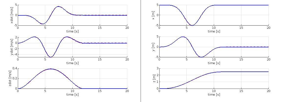
The 3D trajectory result is shown in the figures below.

(Images and codes are from Robotics : Aerial Robotics.)