Here are the assignments for the Robotics Specialization: Computational Motion Planning offered by UPenn on Coursera.
This is the second course in the robotics specialization. Throughout this course, we have gained knowledge on different techniques for planning robot motions. These include graph-based methods, randomized planners, and artificial potential fields.
Graph-based Methods
Graph-based methods tackle the challenge of planning routes for robots in environments with discrete positions, such as grids. To address this problem, we can represent such scenarios as graphs, where nodes signify grid locations, and edges indicate the routes between neighboring grid cells. In this course, we learned and implemented two graph-based algorithms, Dijkstra and the A-Star algorithm.
Dijkstra Algorithm
Dijkstra algorithm is a greedy algorithm for finding shortest path in weighted graphs. Invented by Dutch computer scientist Edsger W. Dijkstra in 1956, Dijkstra’s algorithm has a wide range of applications in computer science, from network routing protocols to GPS nevigation. The algorithm works by exploring all possible paths from a starting node to a target node, keeping track of the distance traveled along each path. It then selects the shortest path and marks it as the optimal route. Here is a pseudocode for the Dijkstra algorithm.
start_node start
for each node v:
    v.dist = infinity
start.dist = 0
list = [start]
while list is not empty:
    current = node in list with smallest distance
    list.del(current)
    for n in current.neighbor:
        if n.dist > current.dist + dist(n, current):
            n.dist = current.dist + dist(n, current)
            n.parent = current
            if n not in list:
                list.append(n)
When the algorithm visits a node, it updates the distances to its neighbors based on the shortest path found so far. Since any new paths to the neighbors would have to go through the current node, the loop invariant is true after updating the distances to its neighbors. When the algorithm terminates, all nodes in the graph have been visited and the loop invariant holds for all nodes. Therefore, the algorithm has found the shortest path from the start node to all other nodes in the graph. With naive implementation, the Dijkstra algorithm has time complexity $\mathcal{O}(|V|^2)$. Using priority queue, this can be reduced to $\mathcal{O}((|V|+|E|)\log(|V|))$.
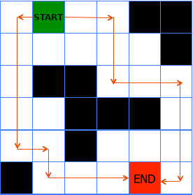
Belowing is a demo result of Dijkstra algorithm implemented in Matlab. The green and yellow block are the start and target position. The blue blocks are the nodes in the list. The red blocks are the nodes with the shortest path have been found and removed from the list.
The Dijkstra algorithm can be computationally expensive on large graphs. Since the algorithm treats all nodes equally and does not consider any heuristic information about the target node, it may explore unnecessary paths. This makes it less suitable for real-time applications.
A-Star Algorithm
To overcome these limitations, the A-Star algorithm was developed by Peter Hart, Nils Nilsson and Bertram Raphael of Stanford Research Institute in 1968. A-Star algorithm enhances Dijkstra’s algorithm by introducing a heuristic function, which provides an estimate of the remaining distance from a particular node to the target node.
The heuristic function needs to satisfy the two criteria:
- $H(goal) = 0$
- For any $x,y\in V$, $H(x)\leq H(y) + d(x,y)$
By those two properties, for any node $v\in V$, we have $$H(v) \leq \text{length of shortest path from v to goal}$$ So the heuristic function $H(v)$ is an underestimate for the distance between the node $v$ and the goal. With the heuristic function, the algorithm chooses the node that is most likely to be on the shortest path between start and goal node.
Here is a pseudocode for the A-Star algorithm.
start_node start, goal_node goal
for each node v:
    v.dist = infinity, v.f = infinity
start.dist = 0, start.f = H(start)
list = [start]
while list is not empty:
    current = node in list with smallest f value
    list.del(current)
    if current == goal:
        return success
    for n in current.neighbor:
        if n.dist > current.dist + dist(n, current):
            n.dist = current.dist + dist(n, current)
            n.f = n.g+H(n)
            n.parent = current
            if n not in list:
                list.append(n)
Belowing is a demo result of A-Star algorithm implemented in Matlab.
Configuration Space Path Planning
Motion planning in configuration space, often referred to as C-space, involves utilizing the C-space as a representation of the feasible motions available to a robot. The configuration space encapsulates all the possible configurations of the robot, including the positions and orientations of its individual components. In configuration space planning, this graph is created directly in the C-space, where each node corresponds to a valid robot configuration and edges represent feasible transitions between them. By navigating this graph, motion planning algorithms can explore the C-space to find collision-free paths for the robot, accounting for its kinematic and dynamic constraints.
For instance, in the case of a two-linked arm, the configuration space would capture all possible combinations of joint angles, allowing the planner to find optimal paths while avoiding collisions. Similarly, in the piano mover’s problem, where a robot needs to navigate through a cluttered environment to move a large object, configuration space planning enables the robot to consider the dimensions and orientations of both the robot and the object, resulting in more precise and accurate path planning. By leveraging the configuration space approach, motion planners can tackle a wide range of challenging scenarios, providing efficient and safe solutions for various robotic applications.
Sampling Methods
In this assignment, we worked with a two-link robot arm and its configuration space. Our goal was to guide the robot arm from one configuration to another while avoiding obstacles in the workspace. We applied collision detection by representing the robot arm and obstacles as collections of triangles. We checked for intersections between these triangles, allowing us to determine if the robot arm would collide with any obstacles while navigating the workspace.
In this example, the workspace and configuration space are shown in the following figure.
We used a freespace sampling method, where we sampled points in the 2-dimensional configuration space and determined whether they were in free space or obstacle space based on the results of the collision check. This allowed us to represent the configuration space obstacles and free space with 2D array and apply the Dijkstra algorithm on torus.
Motion Planning in Free Space
The Dijkstra’s algorithm can be slow in this case, particularly when dealing with a high-dimensional configuration space. To address this, we can employ the A-Star algorithm, which offers a more efficient alternative. The benefits of using the A-Star algorithm, compared to Dijkstra’s algorithm, are illustrated in the figure below.
 |  |
|---|
After finding the shortest path in the configuration space, the robot can proceed to execute the corresponding trajectory.
 |  |
|---|
Sampling-based Methods
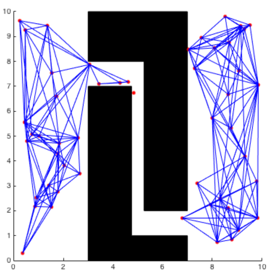
Probabilistic Road Maps
In the above example, we employ a simple approach of evenly discretizing the continuous configuration space and utilizing a graph-based method to determine the shortest path. However, both the Dijkstra and A-Star algorithms can become slow when dealing with a large searching dimension. This situation often arises in scenarios where the configuration space exhibits a high dimensionality. To address this challenge, an alternative method is by selecting points randomly from the configuration space instead of uniformly. By using a subset of these randomly sampled points to represent the free space, we can effectively compute the shortest path. This technique is commonly referred to as Probabilistic Road Maps(PRM). During each iteration of the algorithm, if the randomly sampled point falls in free space, we find k-nearest points according to some distance function. We then try to connect the sampled point to those points using a local planner, which checks if the line between two points is in free space. The pseudocode for the PRM algorithm is outlined below.
Repeat n times:
    Randomly sample a point x in the configuration space
    if x is in free space:
        Find the k closest points to x according to the distance function
        Form a new edge if the connection from x to each point is a free path
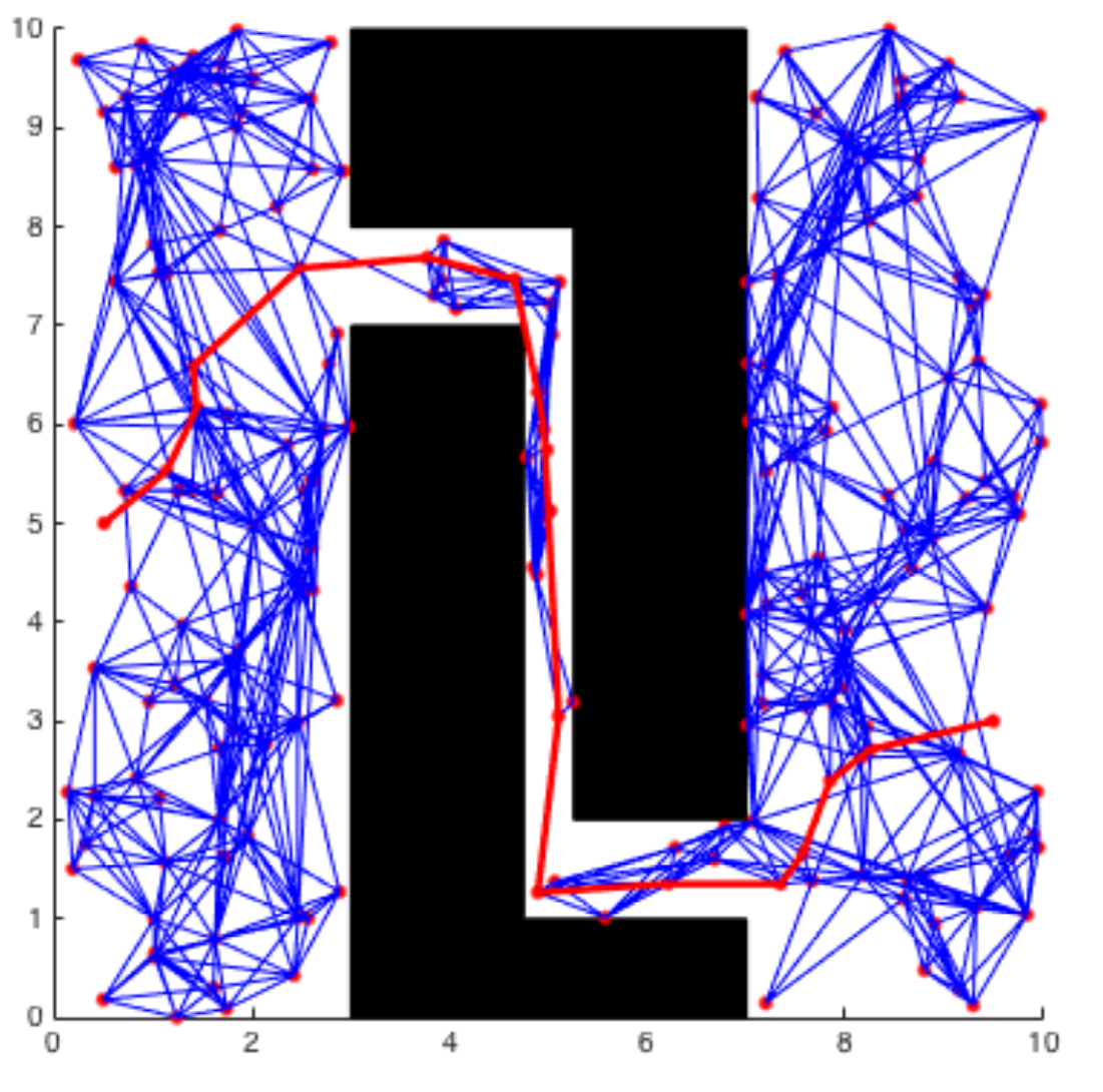
Although sampling-based methods are often effective in practice, it’s important to note that these algorithms are not considered complete. This means that there is a possibility of the algorithm failing to find a path, even if one exists. But we can say that as we continue sampling new points, the algorithm will eventually find a solution if a path to the goal exists. In other word, as the number of samples (n) approaches infinity, the probability of not finding a path approaches zero. This is known as probabilistically complete.
However, this process could take a very long time in some cases. For instance, if we there is a narrow pathway to the goal, the algorithm will require a denser sampling to successfully discover the solution.
 |  |
|---|
Rapidly Exploring Random Trees
The Probabilistic Roadmap (PRM) algorithm offers the advantage of constructing a structure that represents the entire configuration space, allowing for easy adaptation to different starting and ending positions. However, there are scenarios where our focus is solely on a specific pair of starting and goal positions, rather than learning about the entire space. In such cases, the Rapidly Exploring Random Trees(RRT) can be used to construct the path. RRT dynamically explores the configuration space by incrementally building a tree-like structure from a random starting point. It rapidly expands the tree towards unexplored regions, continuously growing and adapting its branches based on sampled points and their connections. This exploration strategy allows RRT to efficiently generate feasible paths that connect a given starting point to an end goal.
Repeat n times:
    Randomly sample a point x in the configuration space
    if x is in free space:
        Find the point y that closest to x
        if (Dist(x,y)>delta)
            find z along the path from x to y such that Dist(z,y) <= delta
            set x = z
        if the connection from x to each point is a free path
            add x to the tree with y as parent
The key idea of the RRT algorithm is to add a point in a random direction and connect it to the closest point in the current tree during every iteration. Thus we expand the tree as much as possible and discover the path from starting point to the goal. In this assignment, we will implement the RPM and RRT for the six-link robot arm.
Since we only sampling points a finite amount of times, the solution is not guaranteed to be optimal. In the figure below, we can observe that the trajectory generated by the RRT algorithm may differ between two runs.
 |  |
|---|
While the RRT algorithm may not provide an optimal solution, it remains valuable in motion planning tasks where finding an exact solution or optimality is not the primary objective. The algorithm strikes a balance between exploration and computational efficiency, making it well-suited for real-time applications where quick and reasonable solutions are desired.
Artificial Potential Field Methods
The artificial potential field method is another approach can be used to guide robots through obstacle environments. The method involves constructing a smooth function over the configuration space as attractive field. The function is designed to have its lowest value at the desired goal location, increasing as the robot moves away. By using the gradient of this function, the robot can be guided towards the goal configuration. Additionally, a repulsive potential field is constructed to steer the robot away from obstacles, based on the distance between the robot and the nearest obstacle. These attractive and repulsive potentials are combined to create a potential function that guides the robot while avoiding obstacles. The gradient of the potential function is then used to determine the direction of motion for the robot.
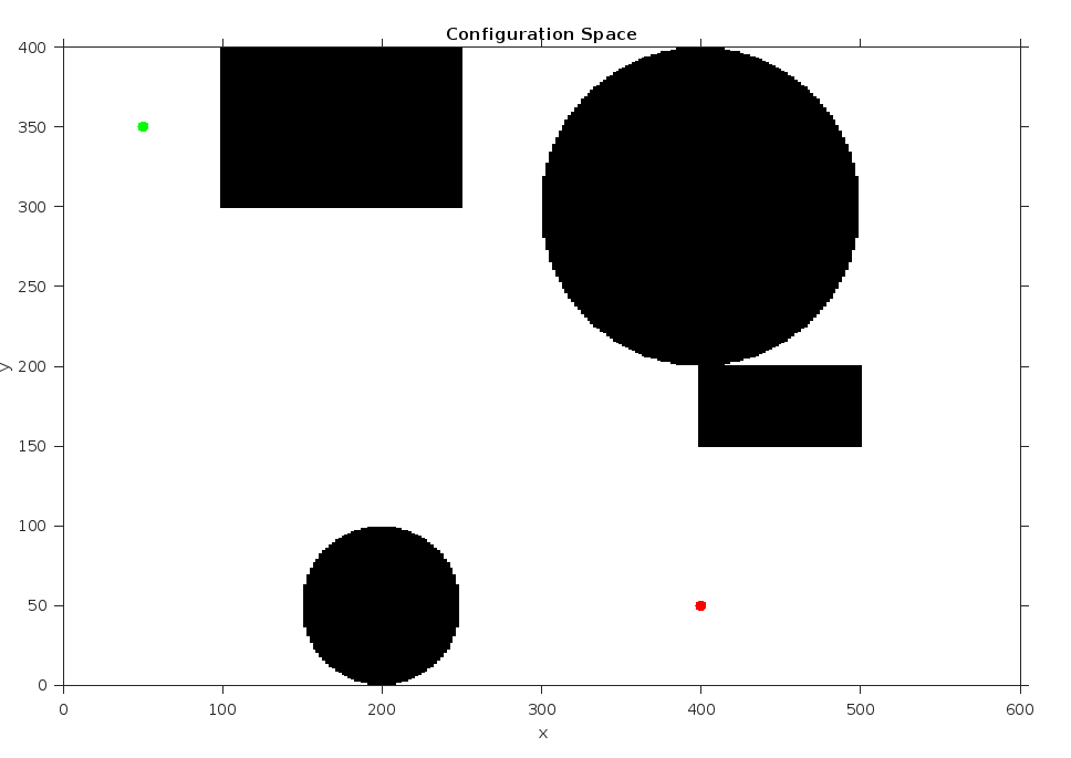
Example
The example demonstrates the motion planning with artificial potential field in a 2D configuration space. The configuration space consists of obstacles represented by black areas, a starting position represented by a green circle, and a goal represented by a red circle. The artificial potential field method is applied to guide the robot from the starting position to the goal while avoiding the obstacles. The potential function is constructed to attract the robot towards the goal and repel it from the obstacles. By evaluating the gradient of the potential function, the robot can determine the direction of motion and navigate towards the goal while circumventing the obstacles.
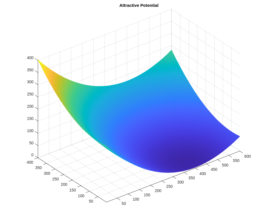
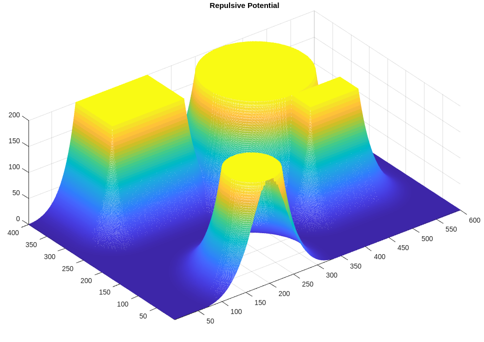
Given the starting and goal position, we can construct the attractive potential field. Then the repulsive potential field can be constructed with the obstacle in the configuration space. The two potential fields are shown below.
 |  |
|---|
Then the overall potential field can be constructed by simply adding those two.
We can depict the path planning on the potential field as a descending process. In the figure below, the red ball represents the current position of the robot, which follows the gradient of the field towards the goal.
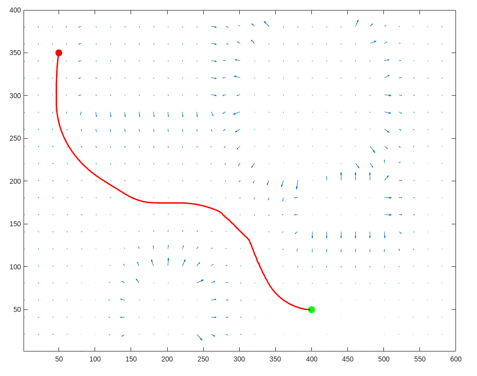
The solution path is illustrated in the quiver plot depicted below. Quiver plots use arrows to represent vectors. In this case, the arrows indicate the direction of the gradient field at different locations in the configuration space, showing the path that the robot follows from the starting position to the goal.
Limitation and Generalization
Issues with Local Minimum
Sometimes, the potential field method can encounter local minima, where it gets stuck and fails to find the correct solution. In such situations, it may be necessary to employ heuristics to identify these cases and switch to alternative methods for motion planning.
Generalization
One way to extend the potential field method to higher dimensions, such as for robots with multiple degrees of freedom, is to consider it as a collection of control points. In the case of a six-link robot arm problem, we can view each joint as a control point and construct a potential field for each control point with respect to its respective goal.
By assigning potential fields to the control points corresponding to the desired goal positions of each joint, we can guide the robot arm towards its overall goal configuration. This generalization allows the potential field method to be applicable to higher-dimensional systems, providing a framework for planning and controlling robots with multiple degrees of freedom.
(Images and codes are from Robotics: Computational Motion Planning.)