Here’s the content from the Robotics Specialization: Estimation and Learning offered by UPenn on Coursera.
This is the fifth course in the robotics specialization. This course is about topics related to machine learning and estimation in robotics.
Gaussian Model Learning
1D Gaussian Distribution
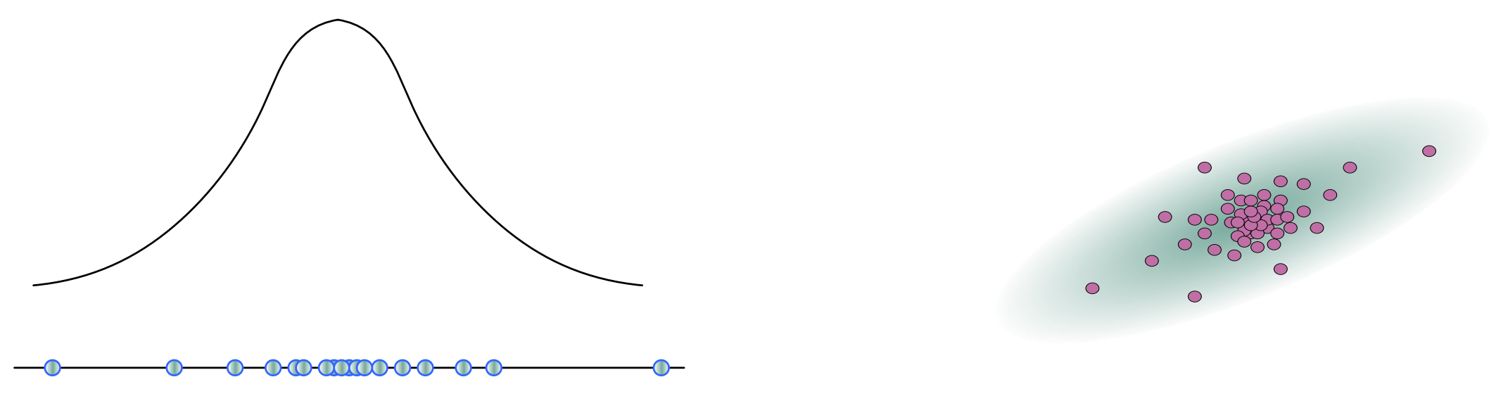
The Gaussian distribution is a widely used probability distribution defined by two parameters, the mean (μ) and standard deviation (σ), which represent its central value and spread. It is characterized by a bell-shaped probability density function (PDF) and has some nice mathematical properties such as the product of two Gaussian distributions is also Gaussian. Additionally, the Central Limit Theorem states that the sum or average of a large number of independent and identically distributed random variables converges to a Gaussian distribution, making it suitable for modeling noise in measurement or uncertainty.
$$ P(x) = \frac{1}{\sqrt{2\pi}\sigma}\exp{\left(-\frac{(x-\mu)^2}{2\sigma^2}\right)} $$
Multivariate Gaussian Distribution
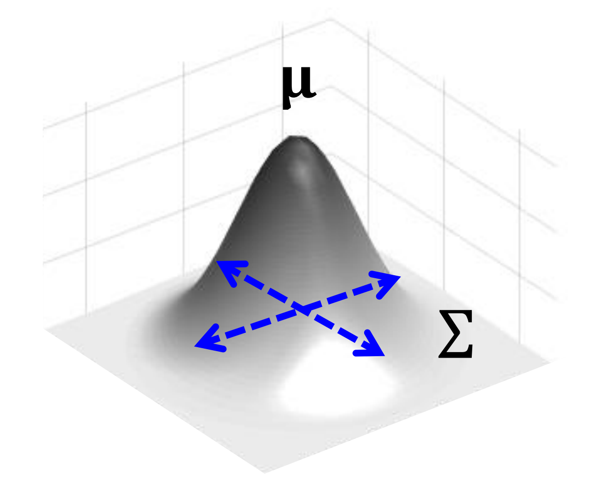
The Multivariate Gaussian is an extension of the 1D Gaussian distribution, allowing us to model complex multidimensional data by specifying a vector of means (μ) and a covariance matrix (Σ) that describes both the central tendency and interrelationships between variables. Just as the one-dimensional Gaussian distribution is characterized by its mean and standard deviation, the multivariate version is defined by these parameters and exhibits a bell-shaped, elliptical probability density function.
$$P(\mathbf{x}) = \frac{1}{(2\pi)^\frac{D}{2}|\Sigma|^\frac{1}{2}}\exp{\left(-\frac{1}{2}\mathbf{(x-\mu)^T\Sigma^{-1}(x-\mu)}\right)}$$
The covariance matrix is a symmetric matrix that describes how pairs of random variables in the distribution are related to each other. It describes both the variances (spread) of individual variables along the diagonal and the covariances (relationships) between pairs of variables off the diagonal. A covariance of zero implies that the variables are uncorrelated. $$ \Sigma = \begin{bmatrix} \sigma_{x_1}^2 && \sigma_{x_1}\sigma_{x_2} \\ \sigma_{x_2}\sigma_{x_1} && \sigma_{x_2}^2 \end{bmatrix}$$
Maximum Likelihood Estimation (MLE)
To determine the most probable parameters for the Gaussian distribution, Maximum Likelihood Estimation (MLE) is often used. For the 1D Gaussian, we want to estimate the mean (μ) and standard deviation (σ). More specifically, we want to find the parameters that maximize the conditional probability over the observational data. $$ \hat{\mu}, \hat{\sigma} = \argmin_{\mu,\sigma} P(\{x_i\}|\mu, \sigma)$$
If we assume each $x_i$ is independently sampled, it becomes:
$$ \hat{\mu}, \hat{\sigma} = \argmin_{\mu,\sigma} \prod_{i=1}^n P(x_i|\mu, \sigma)$$
Next, we can take the natural log of the objective function, since the natural log is a monotonically non-decreasing function.
$$ \hat{\mu}, \hat{\sigma} = \argmin_{\mu,\sigma} \left(\ln \prod_{i=1}^n P(x_i|\mu, \sigma)\right) = \argmin_{\mu,\sigma} \sum_{i=1}^n \left(\ln P(x_i|\mu, \sigma)\right)$$
Then we get the objective function in terms of the following summation.
$$ \hat{\mu}, \hat{\sigma} = \argmin_{\mu,\sigma} \sum_{i=1}^n \left( \frac{(x_i-\mu)^2}{2\sigma^2} + \ln\sigma + \text{const} \right) $$
Take the derivative of the objective function with respect to $\mu$ and $\sigma$, and set them to zero, we get
$$ \hat{\mu} = \frac{1}{N}\sum_{i=1}^N x_i ,\qquad \hat{\sigma}^2 = \frac{1}{N}\sum_{i=1}^N (x_i-\hat{\mu})^2. $$
With similar steps, we can get the MLE solution of multivariate Gaussian distribution.
$$ \hat{\mathbf{\mu}} = \frac{1}{N}\sum_{i=1}^N \mathbf{x_i}, \qquad \hat{\mathbf{\sigma}}^2 = \frac{1}{N}\sum_{i=1}^N (\mathbf{x_i}-\hat{\mathbf{\mu}})(\mathbf{x_i}-\hat{\mathbf{\mu}})^T $$
Mixture of Gaussians
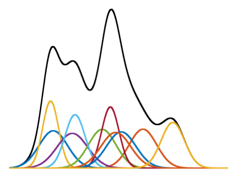
The Gaussian Mixture Model (GMM) extends the Gaussian (normal) distribution to represent complex data distributions by combining multiple Gaussian components. Each component is defined by its own set of parameters, including mean and covariance, allowing GMMs to capture non-symmetric patterns and multimodal data structures.
$$ P(\mathbf{x}) = \sum_{k=1}^K w_k g_k (\mathbf{x}|\mathbf{\mu_k}, \mathbf{\Sigma_k}) $$
The $g_k$ is the Gaussian component with $\mathbf{\mu_k}$ and $ \mathbf{\Sigma_k}$. The $w_k$ is the mixing coefficient with $w_k>0$ and $\sum_{k=1}^K w_k = 1$.
One primary weakness is that GMMs can become computationally demanding when dealing with a large number of components or clusters, as each component introduces additional parameters to estimate, potentially leading to high computational complexity.
Expectation-Maximization (EM) Algorithm
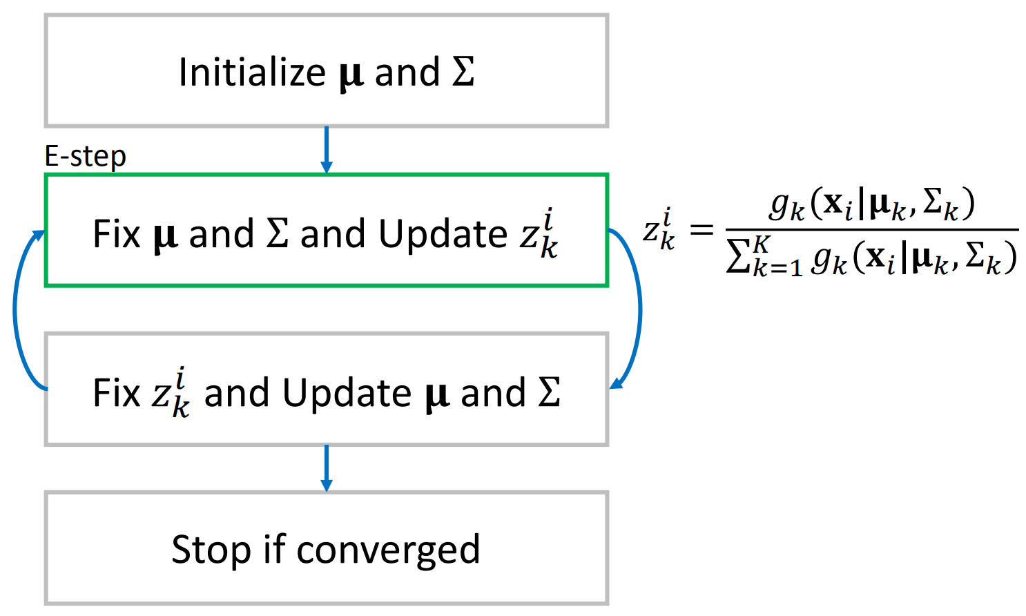
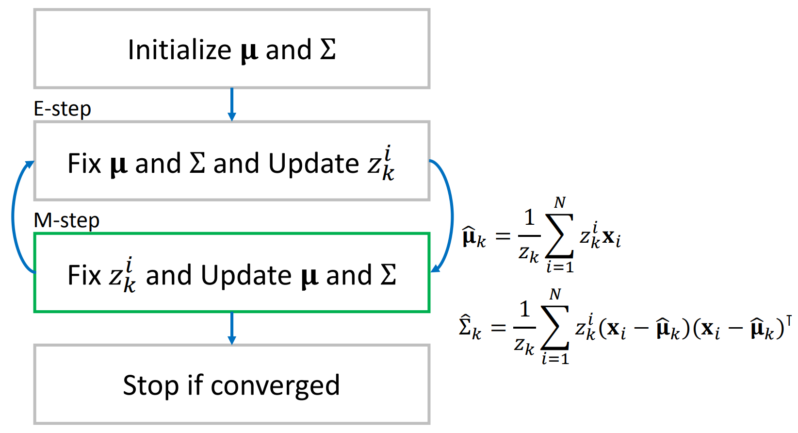
The Expectation-Maximization (EM) algorithm is a computational technique that can be used to estimate the parameters of a Gaussian Mixture Model (GMM). The EM algorithm iteratively updates estimation for the means, covariances, and mixing coefficients of the components. In the Expectation step (E-step), the algorithm computes the expected values of the missing data, given the current parameter estimates. The Maximization step (M-step), then optimizes these parameter estimates based on the expected data. EM iterates between these two steps until convergence. The flowchart below summarizes the updates for the E-step and M-step for estimating GMM parameters.
 |  |
|---|
In the E-step, we fix the parameter of the Gaussian distributions and update the latent parameter $z_k^i = \frac{g_k(x_i|\mu_k,\Sigma_k)}{\sum_{k=1}^Kg_k(x_i|\mu_k,\Sigma_k)}$. Here the latent variable can be interpreted as the probability of $x_i$ is generated from $k$-th distribution. The $z_k^i$ is then fixed in the M-step while the parameters of Gaussian distributions are updated.
Color Learning and Target Detection
In this assignment, we learn to use GMM for target detection using GMM.
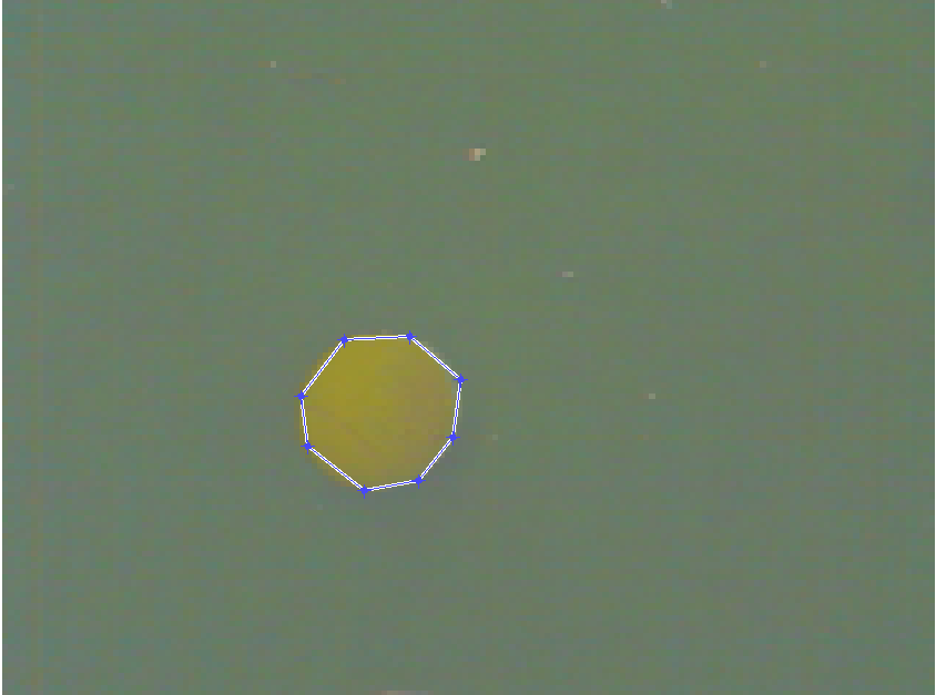
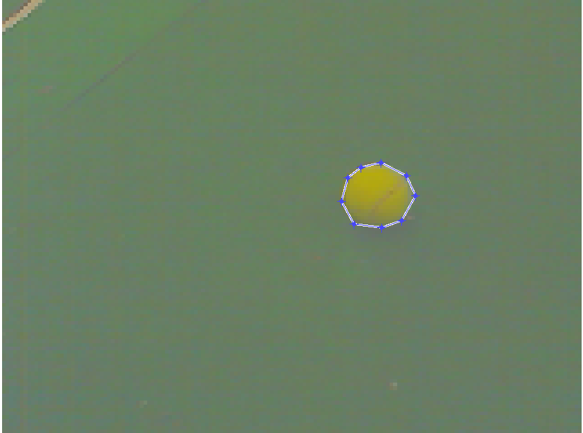
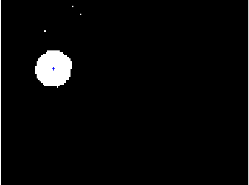
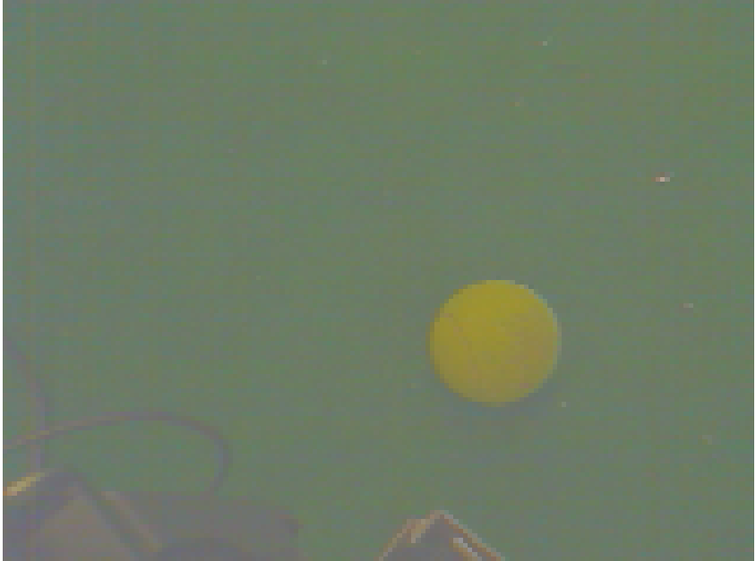
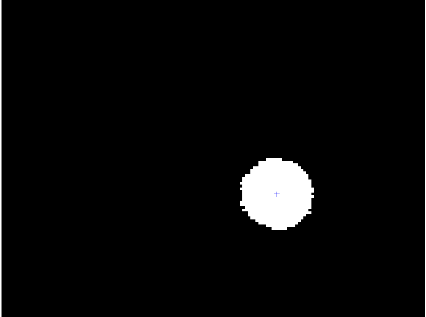
The process of colored ball detection involves two steps. Firstly, we collect color samples of the yellow ball from training images and label them.
 |  |
|---|
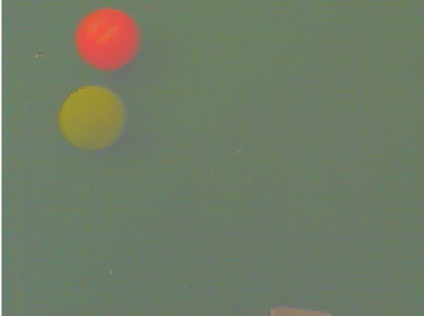
Subsequently, we use this training data to estimate the model parameters, specifically the mean and covariance. Then, during the detection stage, given the model parameters and a test image, we calculate the likelihood of each pixel. Applying an appropriate threshold allows us to obtain a segmentation map of the yellow balls.
 |  |
|---|
 |  |
|---|
Bayesian Estimation - Target Tracking
Kalman Filter Model
Kalman filtering is a powerful algorithm that can the parameters of interest for dynamic systems. For example, the kalman filter can be used for tracking position of an object given a series of noisy measurements.
In this section, we consider a linear dynamic system of an object moving in the 1D space. Let $x_t$ be the state vector of the object and $z_t$ be the noisy measurement of $x_t$.
$$ x_t = \begin{bmatrix} s & \frac{ds}{dt}\end{bmatrix} \qquad z_t = Cx_t.$$
The dynamic of the object is described by the transition matrix $A$.
$$ x_{t+1} = Ax_t + B u_t \qquad A = \begin{bmatrix} 1 & dt \\ 0 & 1 \end{bmatrix} $$
where $u_t$ represents all the external inputs that not depends on $x_t$.
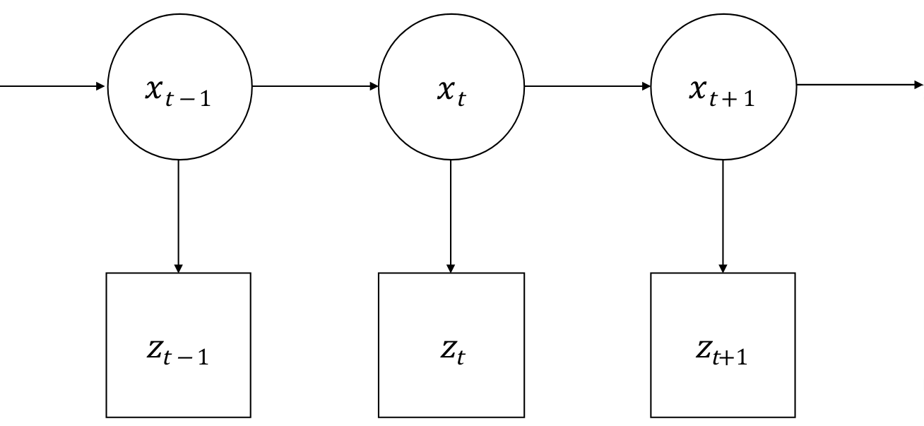
Since we can only estimate the state from the estimation of previous state and noisy measurement, we need to capture the uncertainty in our estimation. Using Baysian modeling, we can characterize the uncertainty with conditional probabilities:
$ p(x_{t+1}|x_t)$ represent the prediction of the current state given the previous state, $ p(z_t|x_t)$ represent the probablity of measurement given the state, and the state vector can be modeled with a Gaussian distribution $ p(x_t) = \mathcal{N}(x_t, \Sigma_t)$.
Combining the probability model and the previous linear dynamic model, we can get the following.
$$ p(x_{t+1}|x_t) = A p(x_t) + \nu_m = A\mathcal{N}(x_t, \Sigma_t) + \mathcal{N}(0, \Sigma_m), $$ $$ p(z_t|x_t) = C p(x_t) + \nu_o = C\mathcal{N}(x_t, \Sigma_t) + \mathcal{N}(0, \Sigma_o),$$
where $\nu_m$ and $\nu_o$ are the noise of estimation modeled by zero mean Gaussian distributions.
Then apply the linearity and summation of Gaussian distributions.
$$ p(x_{t+1}|x_t) = \mathcal{N}(Ax_t, A\Sigma_tA^T) + \mathcal{N}(0, \Sigma_m) = \mathcal{N}(Ax_t, A\Sigma_tA^T + \Sigma_m)$$ $$ p(z_t|x_t) = \mathcal{N}(Cx_t, C\Sigma_tC^T) + \mathcal{N}(0, \Sigma_o) = \mathcal{N}(Cx_t, C\Sigma_tC^T + \Sigma_o)$$
MAP Estimate of KF
After building the probabilistic model for the states and observations, we want to find the posterior distribution of the object given the previous state and observations.
$$ p(x_t|z_t, x_{t-1}) = \frac{p(z_t|x_t, x_{t-1}) p(x_t|x_{t-1})}{p(z_t)}$$
Here $p(z_t|x_t, x_{t-1}) = A\mathcal{N}(x_t, \Sigma_t) + \mathcal{N}(0, \Sigma_m)$ is the prior distribution of the object state at time $t$. And $p(z_t|x_t) = C\mathcal{N}(x_t, \Sigma_t) + \mathcal{N}(0, \Sigma_o)$ is the likelihood. We can use the Maximum A Posteriori (MAP) to get a better estimation for $x_t$.
$$ \hat{x}_t = \argmax _{x_t} p(x_t|z_t, x _{t-1}) = \argmax _{x_t} p(z_t|x_t, x _{t-1}) p(x_t|x _{t-1})$$
$$ \hat{x}_t = \argmax _{x_t} \mathcal{N}(Cx_t, C\Sigma_tC^T + \Sigma_o) \mathcal{N}(Ax_t, A\Sigma_tA^T + \Sigma_m)$$
Take logorithm on both sides and using the following substitution for simplificiation.
$P = \Sigma_t = A\Sigma_{t-1}A^T + \Sigma_m, \quad R = C\Sigma_tC^T +\Sigma_o$
Then we have $$ \hat{x}_t = \argmin _{x_t} (z_t -Cx_t)R^{-1}(z_t-Cx_t) +(x_t-Ax _{t-1})P^{-1}(x_t -Ax _{t-1}).$$
Taking the derivative with respect to $x_t$, and apply the Matrix Inversion Lemma, we can get the posterior estimation
$$ \hat{x}_t = Ax _{t-1} + K(z_t -CAx _{t-1}) ,$$
where $K = PC^T(R+CPC^T)^{-1}$ is known as the Kalman gain.
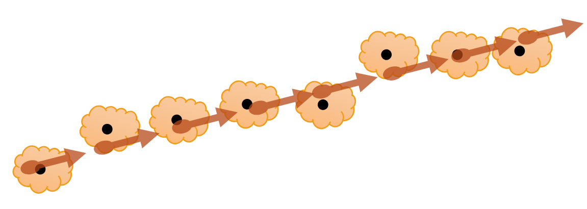
For the exercise in this section, we learned to implement a Kalman filter for ball tracking in 2D space.
Mapping
Occupancy Grid Mapping
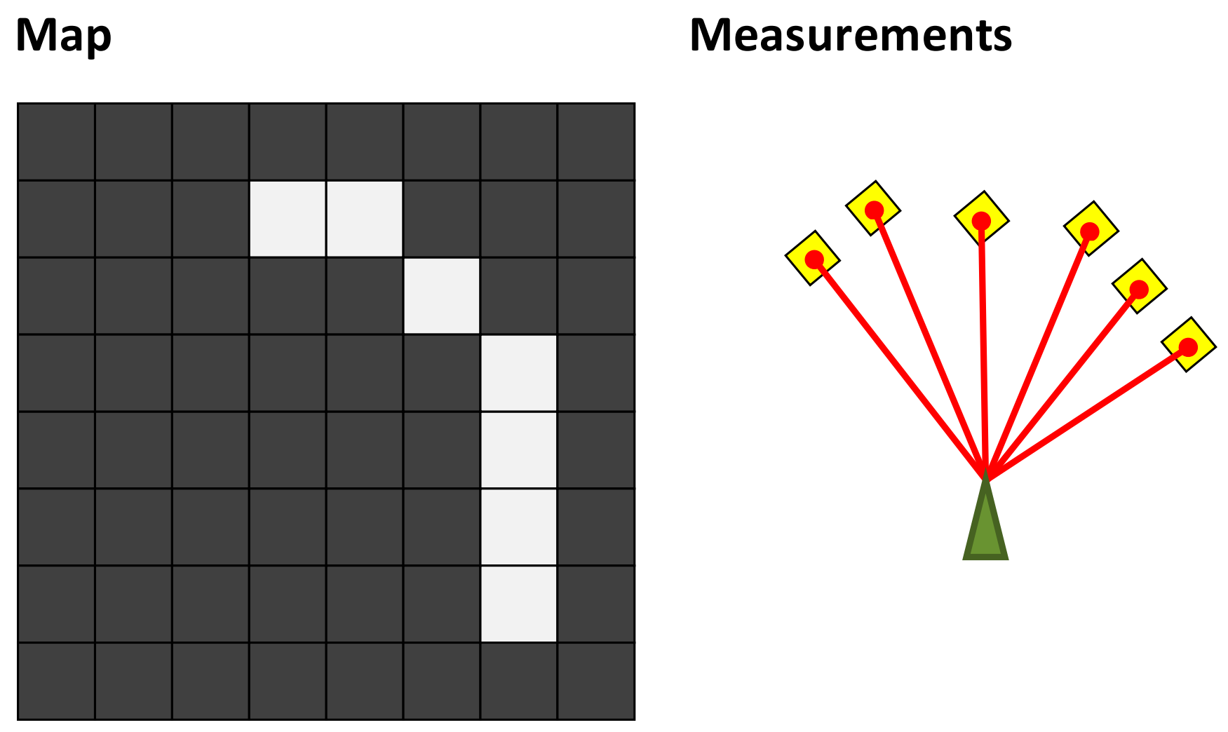
It is critical for mobile robots to know the surrounding environments. For the mobile robot moving in the 2D space, an intuitive way to describe the environment is Occupancy Grid Mapping, which represent the environment with a grid map. In general, there are two binary random variable associated with each cell in the grid map: the occupancy $m_{x,y}:\{free, occupied\} \rightarrow \{0,1\}$ and the measurement $z\sim \{0,1\}$.
The measurement can be obtained by the range sensor, which detect the obstacles in the path of rays. To characterize the uncertainty in the measurement, we can model the measurement using the conditional probability.
$$\begin{align*} &p(z=1|m_{x,y}=1) \quad \text{True occupied measurement} \\ &p(z=0|m_{x,y}=1) \quad \text{False free measurement}\\ &p(z=1|m_{x,y}=0) \quad \text{False occupied measurement}\\ &p(z=0|m_{x,y}=0) \quad \text{True free measurement} \end{align*}$$
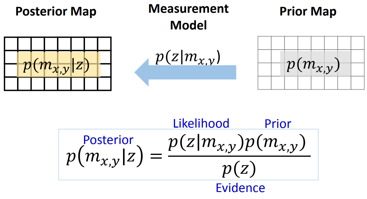
Given our prior belief of the map and the measurement model, we can find the posterior map using Bayes’ rule.
To simplify the map update process, we can represent the map using log-odd values. The Odd of an event is defined as the ratio between the probability of the event happens and probability of the event not happens. In this case, the Odd is defined as following.
$$ \begin{align*}Odd((\text{grid is occupied given z}) &= \frac{p(m_{x,y}=1|z)}{p(m_{x,y}=0|z)} \\ &= \frac{p(z|m_{x,y}=1)p(m_{x,y}=1)}{p(z|m_{x,y}=0)p(m_{x,y}=0)} \\ \log Odd &= \log\frac{p(z|m_{x,y}=1)}{p(z|m_{x,y}=0)} + \log \frac{p(m_{x,y}=1)}{p(m_{x,y}=0)}\end{align*}$$
The first term is the log-odd of the measurement, and the second term is the log-odd of the prior map. At each time $t$, we can use log-odd update to get posterior map of the occupancy grid map by adding the new measurement to the current map.
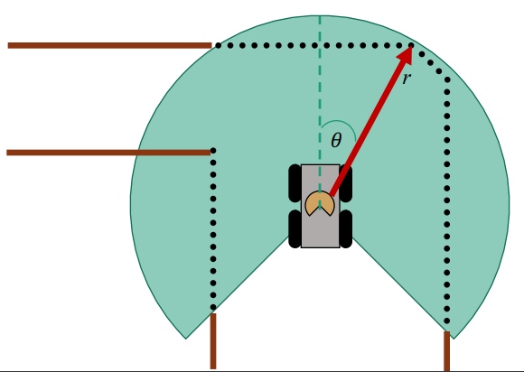
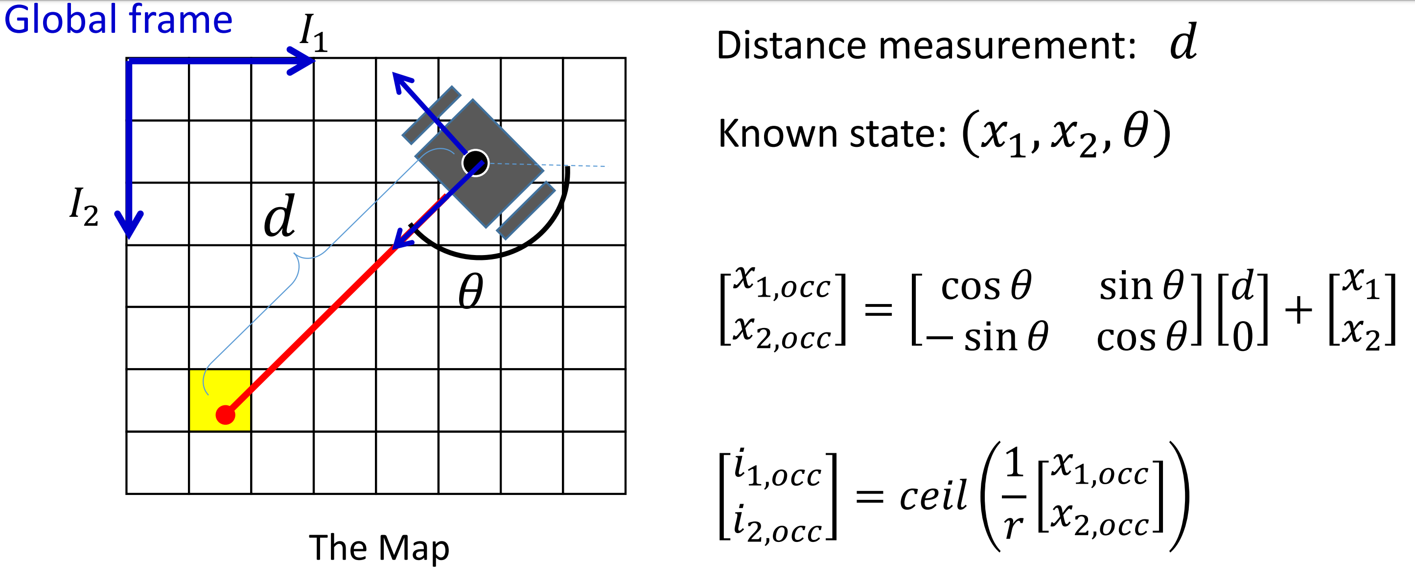
In addition, we need to discretize the continuous value from distance sensor to the grid map. Given the size of grid $r$, the index of each cell is given by $i=ceil((x-x_{min})/r)$.
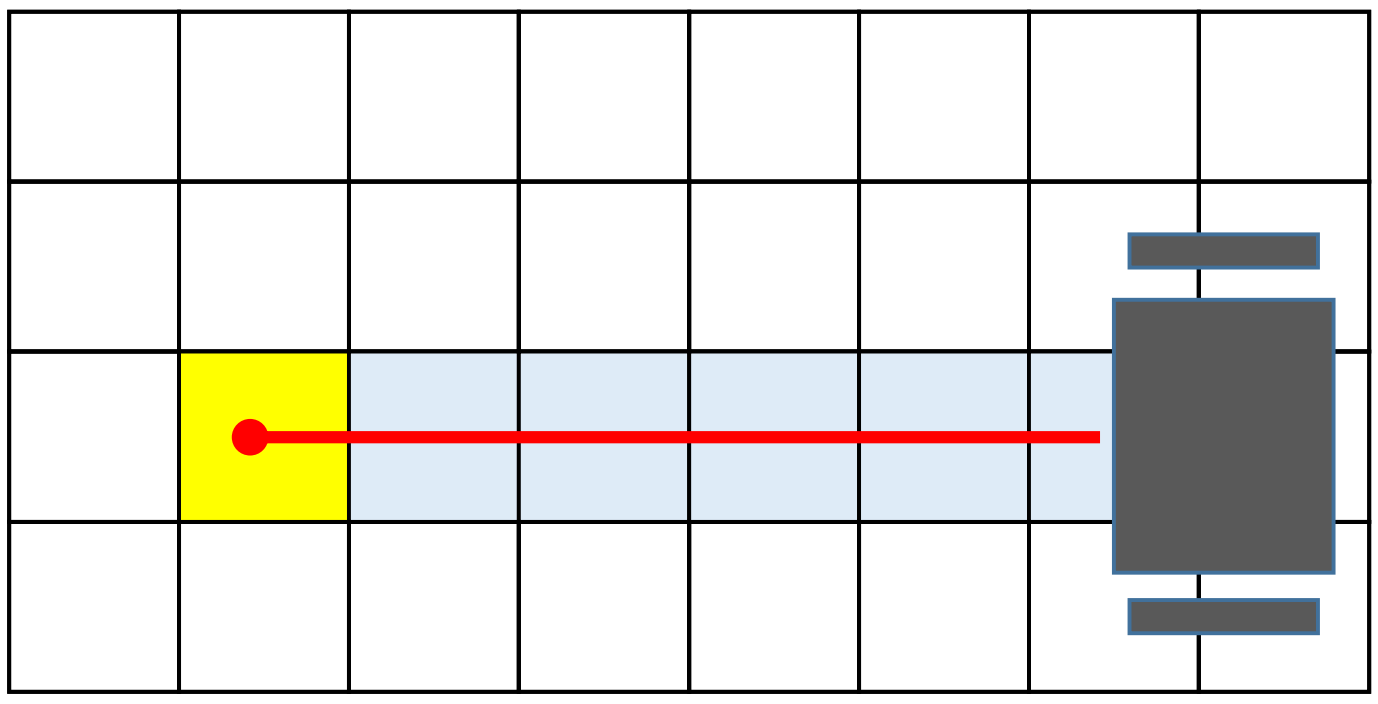
In practice, given the global frame of the map $(X_1, X_2)$ and the body frame of the robot at $(x_1, x_2)$ with orientation $\theta$ and distance measurement $d$. We can relate the sensor measurement to the robot map using the rotation matrix.
$$ \begin{bmatrix} x_{1,occ} \\ x_{2,occ} \end{bmatrix} = \begin{bmatrix} \cos\theta & \sin\theta \\ -\sin\theta & \cos\theta \end{bmatrix}\begin{bmatrix} d\\ 0 \end{bmatrix} + \begin{bmatrix} x_1 \\ x_2\end{bmatrix} $$
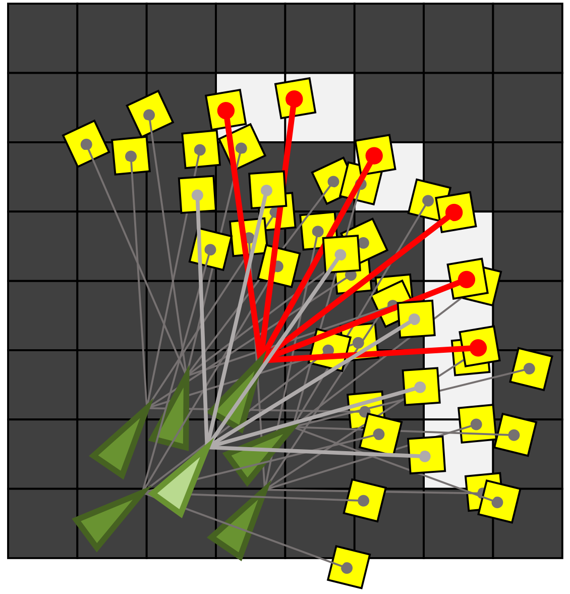
After finding occupied cell $(x_{1,occ}, x_{2,occ})$ from the distance sensor, we can use the Bresenham’s line algorithm to calculate the index of the free cells. Often we will have multple range measurements from a robot. In that case, we can use the procedure described above to find occupied and free cells for each ray and update the map.
In the assignment, we apply the method discuss above to compute the map given the range data from lidar.
3D Mapping
To build a 3D map of environment, we can use sensors such as 3D range sensor, stereo camera, or depth camera to capture the 3D coordinate of the distance measures. One challenge of extending the 2D mapping method to 3D is the representation of the map. The occupancy grid map is not suitable in 3D case because empty space will be significantly large in 3D space compares to the occupied space. So there will be information losses in the discretization steps. And it is also not a memory efficient way to represent the map for the same reason.
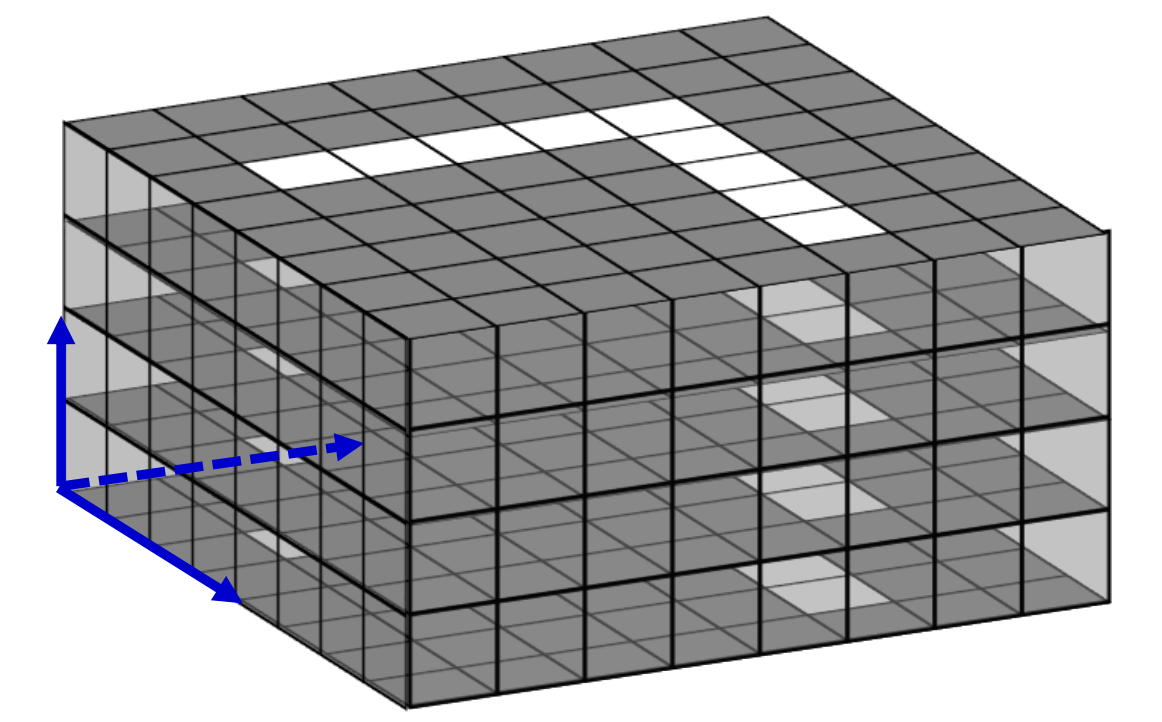
The list representation of measured points is more efficient to represent map in 3D space, and it does not involves the discretization challenge. However, the number of points increase quickly as the map getting large, and it will take a long time to access or check the existing points in the map.
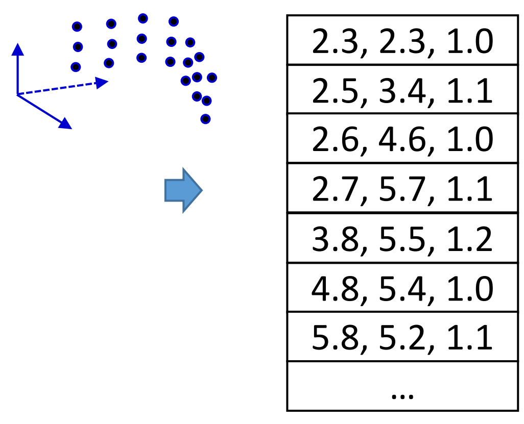
To overcome this issue, we want to find some structured way such as trees to represent the data in a list, so that we can access the existing data ponints quickly while maintan the sufficiency of the memory usage.
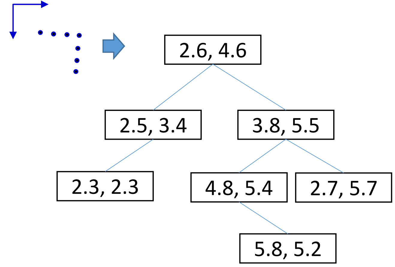
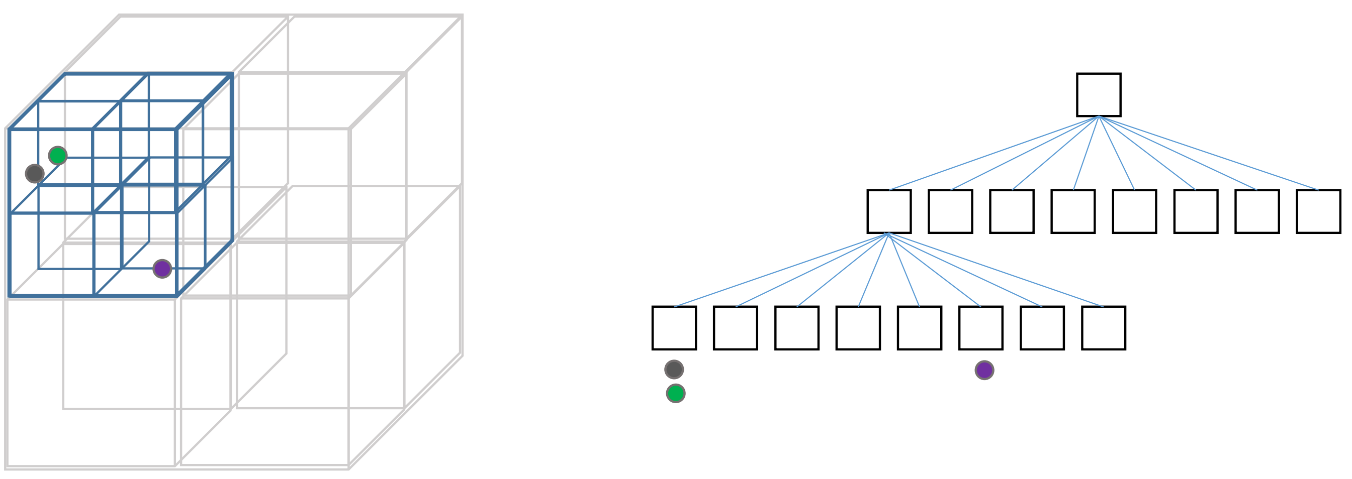
An example of such method is called Octree. An octree is a tree data structure used for partitioning 3D space by recursively subdividing it into eight octants. Each node in an octree represents a cubic region of space and can have up to eight children, corresponding to the eight subdivided regions. Octrees help optimize operations such as collision detection, visibility determination, and rendering by reducing the complexity of spatial calculations, enabling faster and more efficient processing of 3D data.
Localization
Odometry Modeling
In the previous section, we assume the position of the robot relative to the map is known from the data. The position of robot can be obtained through various methods such as GPS, Cell towers, Wifi hotspots, which provide an absolute coordinate of the robot. However, these positioning systems have different levels of accuracy due to the noisy of measurement. In many cases, the accuracy of the positioning system may not satisfies the requirement of the application such as robot navigation or self-driving car. On the other hand, the local information of the robot usually can be obtained with more precision, therefore can be integrated to get more accurate localization.
An simple example of odometry is the wheel encoder of mobile robot. Wheel encoders measure the rotation of the robot’s wheels, allowing the calculation of the distance traveled based on the wheel’s size. By tracking the rotation of each wheel over time, the robot’s movement can be estimated. This information can then be combined with data from other sensors such as Gyroscope to improve the overall accuracy of the robot’s position estimate.
Map Registration
In the localization problem, we have two sets of information: the map of environment, and the measurement from the robot. We need to register the local measurement from the robot to the known map.
The goal is to find the pose of the robot that best fit to the measurements. The odometry information provide a set of belief states that we can search over. More specifically, we want to maximize the correlation between laser obstacles and map obstacles, as well as the free spaces in the laser measurements and map. Next section we introduce the particle filter for modeling the pose of the robot given measurements.
Particle Filters
The particle filter represents a distribution with a set of samples (particles) instead of explicit parametric form.
For the localization problem, each particle is a pair of values pose and weight, where weight represent the confidence of the pose. Similar to the Kalman filter, during the robot motion, we update the particle given the odometry information.
During the initial stage, often most of the particles have very small weights and do not provide useful information for the pose of robot. We can use the resampling process the make the particles better represent the distribution of the robot pose. The number of effective particles $n = (\sum w_i)^2/ \sum w_i^2$ can be used as a criterion for resampling. In brief, the resampling process will make the prune out lower weighted particles.
Iterative Closest Point
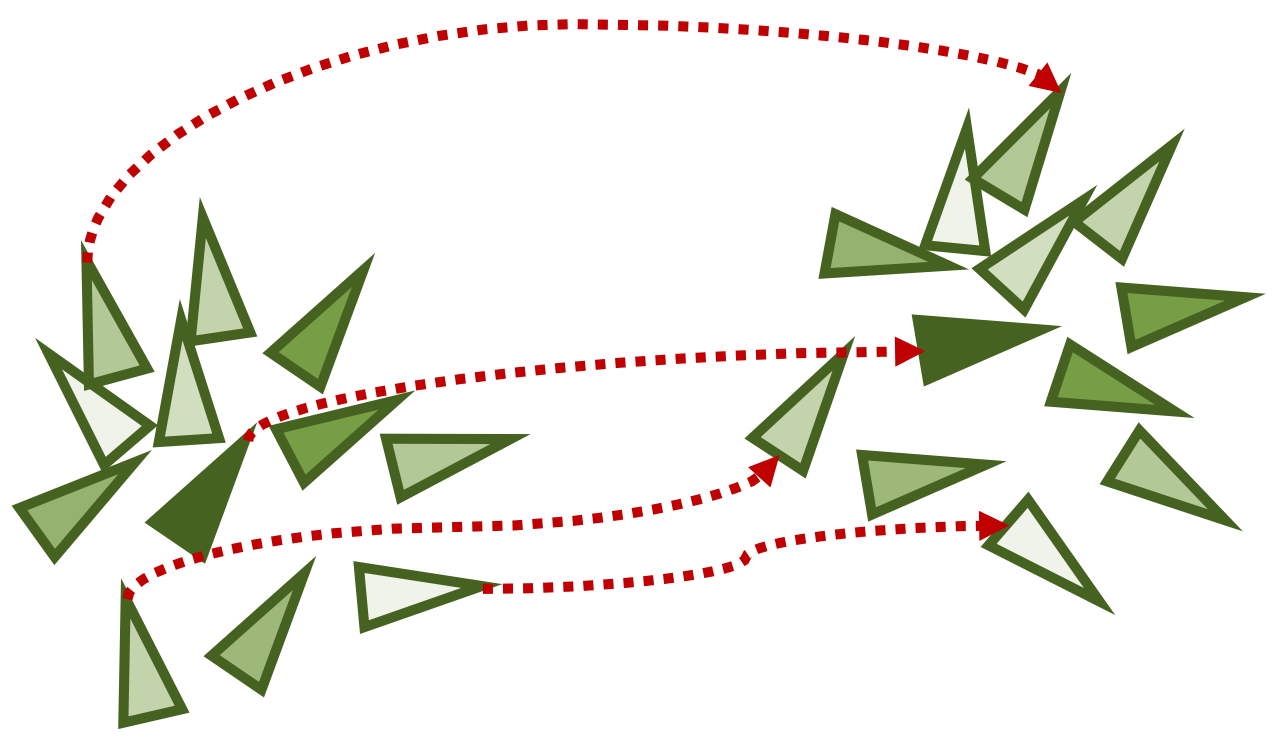
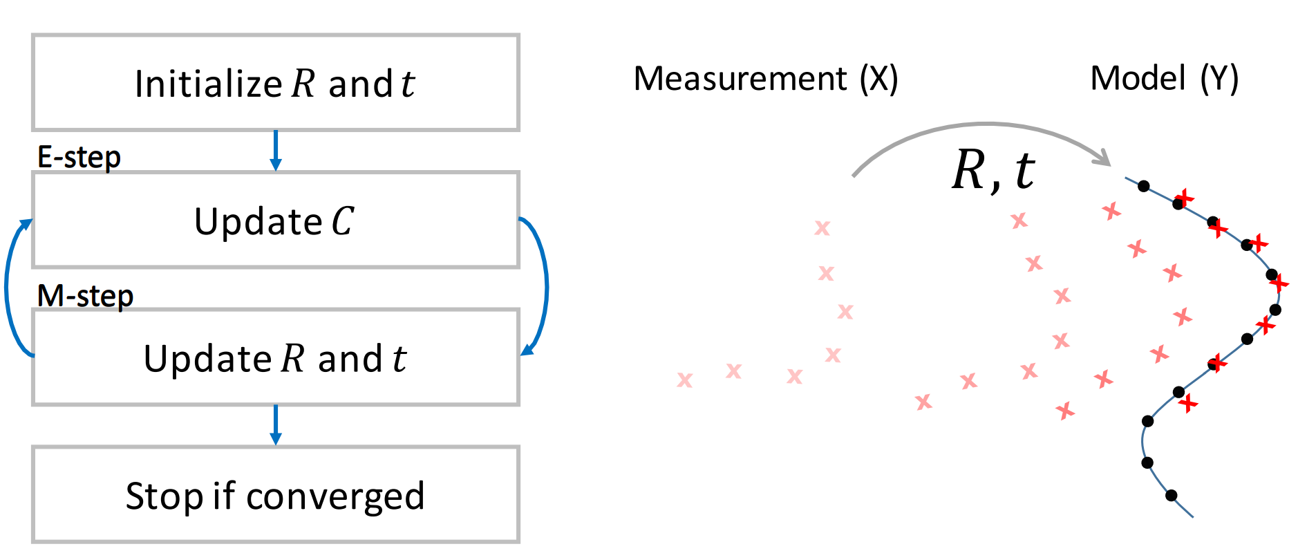
The particle filter is not suitable in 3D space. Since the pose has six degree of freedom, it requires exponentially more points to be sampled compares to the ground mobile robot. An alternative way to register the map is to match the observation points to the map directly. This can be done using the Iterative Closest Point (ICP) algorithm. In general, ICP algorithm can be used to register two point sets $X$ and $Y$. This involves solving two problems: finding the translation and rotation between two points, and determine the correspondences between points.
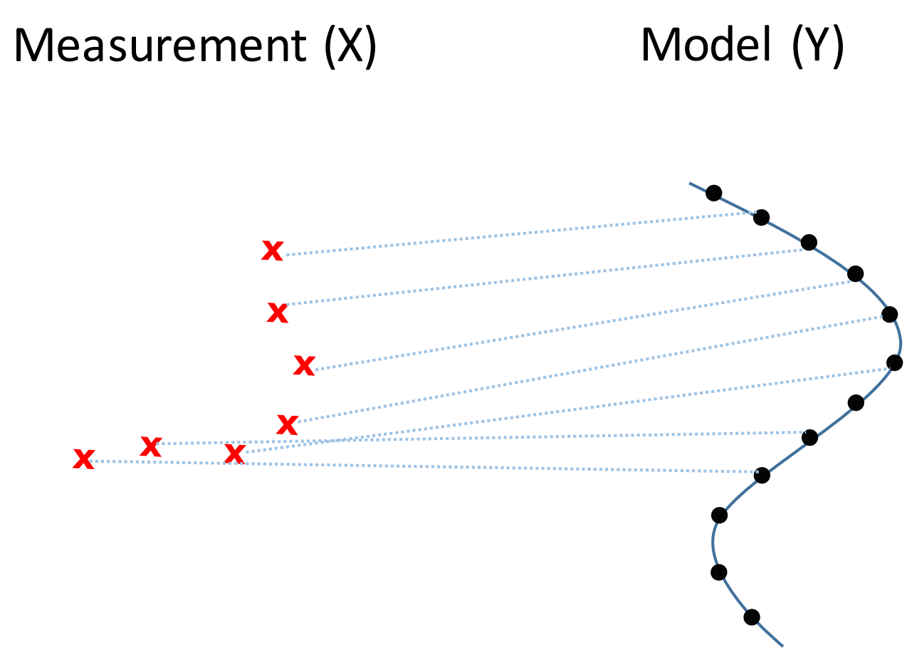
We can use the EM algorithm to solve these two problem iteratively. In the E-step, we find the closest points of all measured points corresponding to the map. And in the M-step, we fix the point correspondence and find the translation and rotation that better match the two point sets. The algorithm will improve the registration of the points in each iterations. And we can repeat this steps until it converges. Since the convergence only on the local minimum, we should assumes the two points sets are close enough at the beginning. The ICP algorithm is suitable for computing the motion increment of the robot.
(Images and codes are from Robotics: Estimation and Learning.)