Here’s the content from the Robotics Specialization: Perception offered by UPenn on Coursera.

This is the fourth course in the robotics specialization. Throughout this course, we learn the basics of computer vision that involve robotics.

Single-view Geometry

Pinhole Camera

The pinhole camera is the most commonly used camera model for computer vision. It can be seen as a simple form of perspective projection as shown in the figure below, which refers to the way objects in a three-dimensional scene appear on a two-dimensional surface when viewed from a particular point or viewpoint. The image below shows a 2D example. The rays from an object converge to some points in the image plane. Here $Y$ is the height of the object in the scene and $y$ is the height of the object in the image plane, $Z$ is the distance of the object from the camera, and $f$ is the focal length.

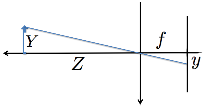
The geometry of the pinhole camera model imposes the following constraint

$$ \frac{Y}{Z} = -\frac{y}{f}. $$

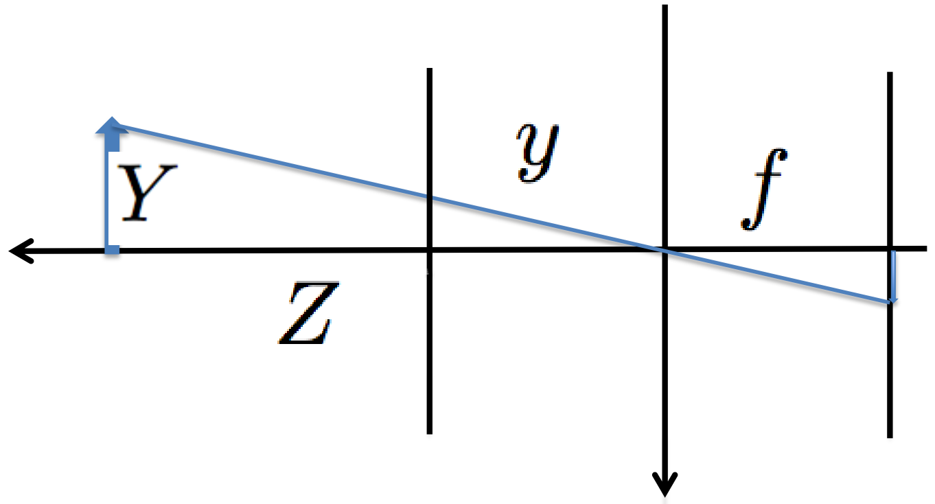
If we assume the image plane is in front of the lens, then we have the following expression to transform a measurement in the scene to coordinates in the image.

$$ y = f\frac{Y}{Z}. $$

Homogeneous Coordinate

An interesting problem in computer vision that involves perspective projection is the transformation of the three-dimensional world into a two-dimensional image. There are two fundamental concepts called vanishing point and vanishing line. The vanishing points are the points on that line where parallel lines from the scene converge, giving the illusion of depth and distance. The vanishing line is a horizontal line on the image plane that represents the viewer’s eye level. It serves as a reference for the convergence of parallel lines in the scene.

The figure below shows two vanishing points at the horizon line and vertical vanishing points at infinity.

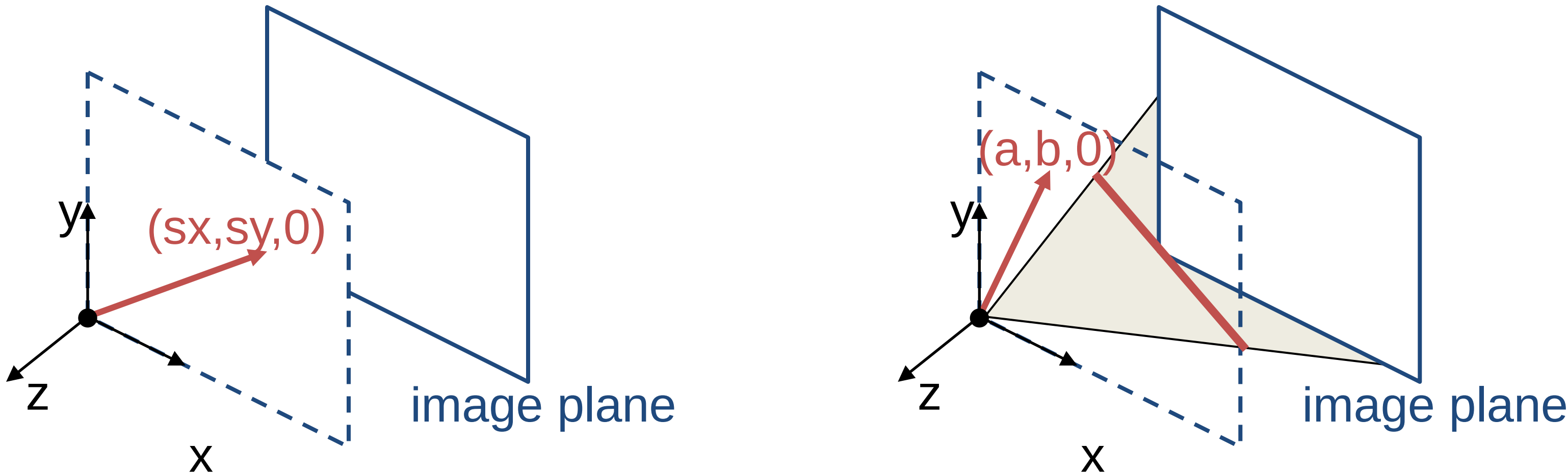
Homogeneous coordinates are often used to represent both finite and infinite points and lines in the image. In addition, homogeneous coordinates make transformations, like rotation and translation more efficient to compute. In the homogeneous coordinates, each point in the image is a ray in projective space.

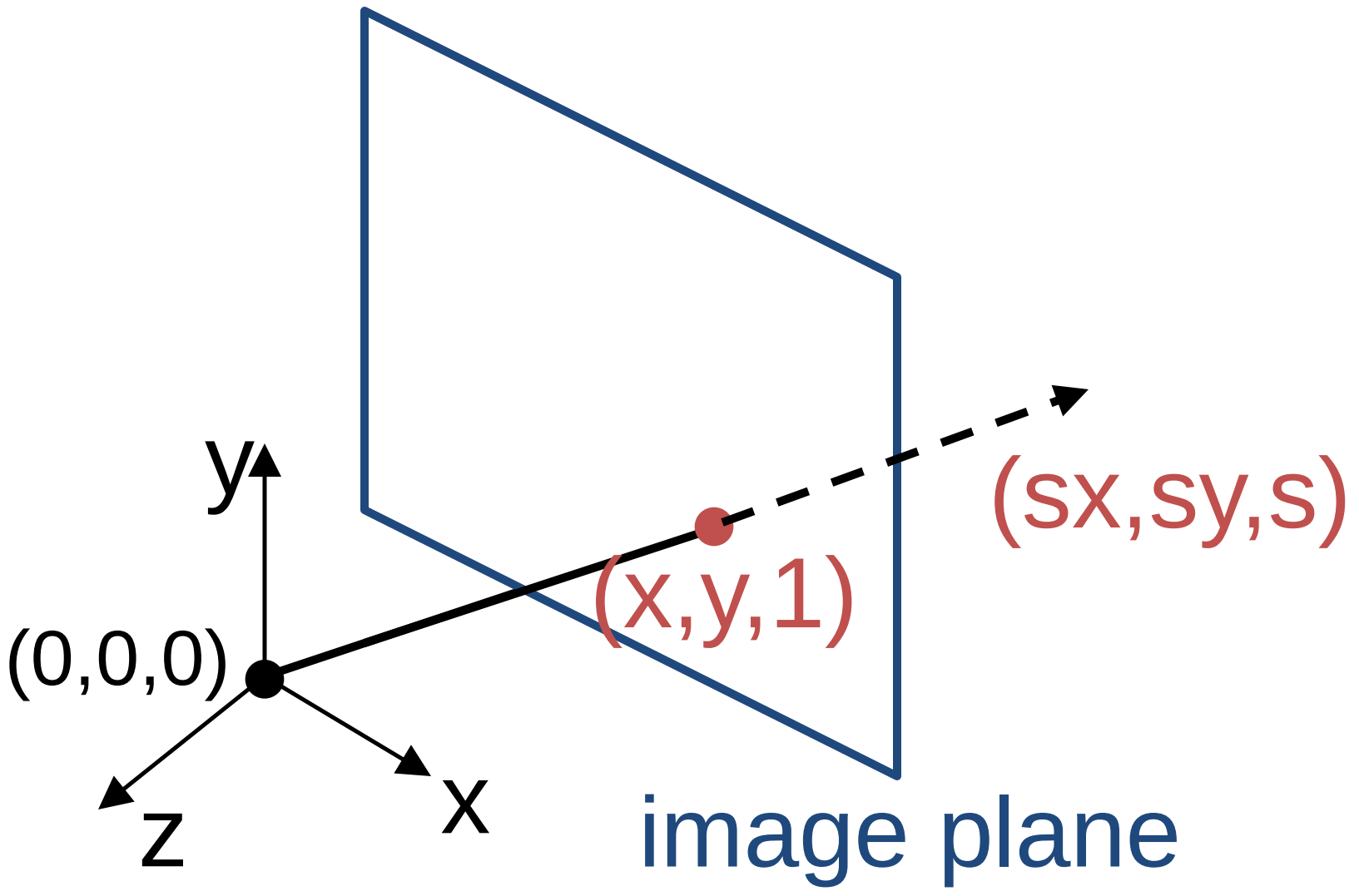
In the above figure, Each point $(x,y)$ on the plane is represented by a ray $(sx,sy,s)$. Since all points on the ray are equivalent, the homogeneous representation of the point is $(x, y, 1) \approx (sx, sy, s)$.

$$ \begin{bmatrix} x\\ y \end{bmatrix} \xrightarrow[\text{coordinates}]{\text{homogeneous}} \begin{bmatrix} x\\ y \\ 1\end{bmatrix} $$

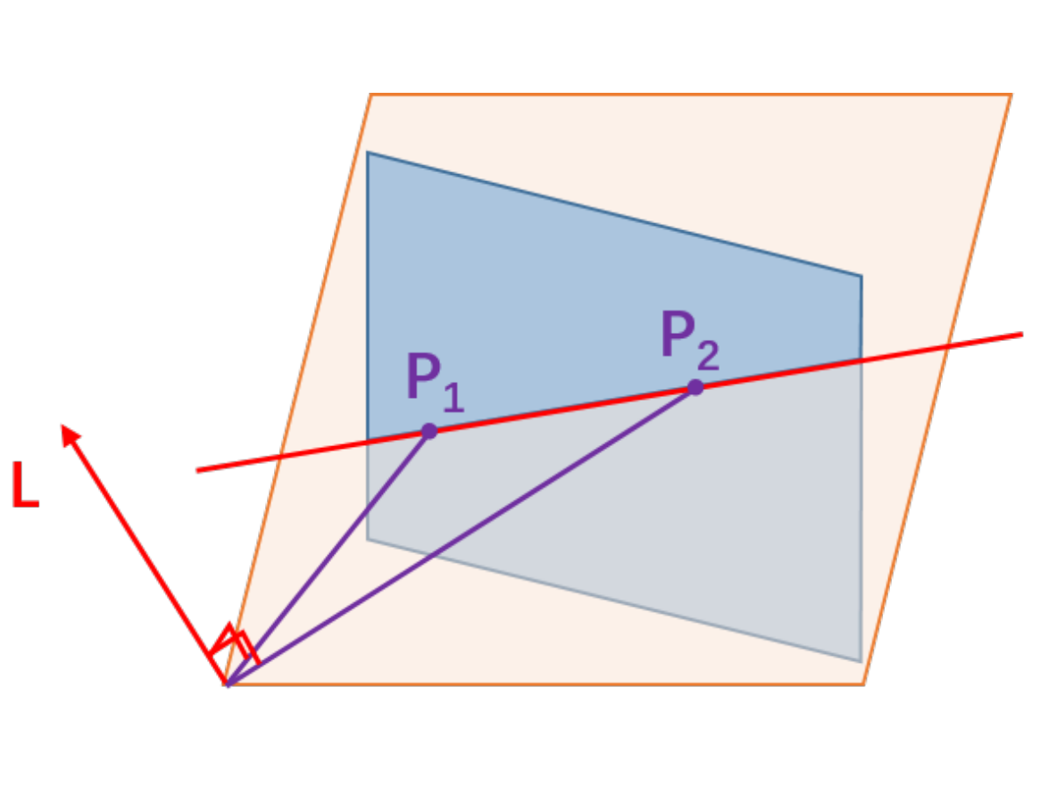
Similarly, the line is a plane of rays through the origin as shown in the figure below.

If $(a,b,c)$ is the surface normal of a plane, a line is all the rays $(x,y,z)$ satisfying the following equation. $$ax + by + cz = 0$$

The homogeneous representation of a line can be defined as the normal of that plane $(a,b,c)$. The line $(0,0, 1)$ represents the line at infinity.

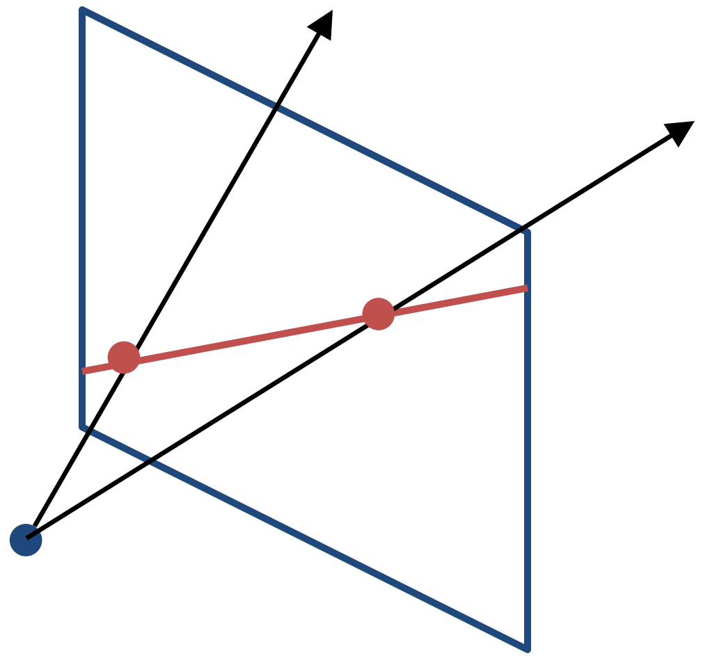
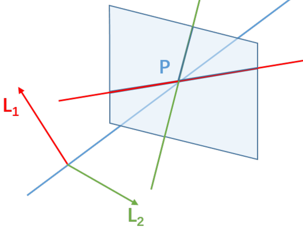
Given two points $P_1$ and $P_2$, the line passing through both points is defined by $l=P_1 \times P_2$. Similarly, the point at the intersection of two lines can be represented by the cross product of two lines $P = l_1\times l_2$. This is called point-line duality.

In this homogeneous coordinate, we can represent the line at infinity as $(0, 0, 1)$. This encapsulates the concept of lines that are parallel in Euclidean space but intersect at infinity in the projective plane. Similarly, ideal points at infinity can be defined as (x, y, 0). The point/line at infinity is also known as the ideal point/line.

Rotation and Translation

Homogeneous coordinates are also valuable in expressing transformations between different coordinate frames. This scenario commonly occurs in many robotics applications. For instance, consider a point $P$ that can be represented in both the camera frame $^cP$ and the world frame $^wP$. The transition between these two coordinate frames can be effectively captured using a rotation matrix $^cR_w$ and a translation matrix $^cT_w$.

$$ {}^cP = {}^cR_w {}^cP +{}^cT_w$$

In homogeneous coordinates, we can write the rotation and translation matrix as a single compact transformation matrix.

$$ {}^cM_w = \begin{bmatrix} & {}^cR_w & & {}^cT_w \\ 0& 0& 0 & 1 \end{bmatrix} $$

Intrinsic Parameters

Recall the relationship between image coordinates and world coordinates. $$y = \frac{fY}{Z}$$ $$x = \frac{fX}{Z}$$

This can be expressed in the matrix form.

$$Z\begin{bmatrix}x\\ y\\ 1\end{bmatrix} = \begin{bmatrix}f & 0 & 0 \\ 0 & f & 0 \\ 0 & 0 & 1 \end{bmatrix} \begin{bmatrix}X\\ Y\\ Z \end{bmatrix}$$

Let $p_x$, $p_y$ denote the principle point, where the optical axis hits the image plane. And $\alpha_x$, $\alpha_y$ are the pixel scaling factor. We have the following relationships.

$$\begin{bmatrix}x\\ y\\ z\end{bmatrix} = \begin{bmatrix}\alpha_x & s & p_x \\ 0 & \alpha_y & p_y \\ 0 & 0 & 1 \end{bmatrix} \begin{bmatrix}f & 0 & 0 \\ 0 & f & 0 \\ 0 & 0 & 1 \end{bmatrix} \begin{bmatrix}X\\ Y\\ Z \end{bmatrix}$$

$$\begin{bmatrix}x\\ y\\ z\end{bmatrix} = \begin{bmatrix}f_x & s & p_x \\ 0 & f_y & p_y \\ 0 & 0 & 1 \end{bmatrix} \begin{bmatrix}X\\ Y\\ Z \end{bmatrix} $$

Here $s$ is a parameter that accounts for the image plane that is not normal to the optical axis. We can also represent the pixel coordinate $u_x$, $u_y$ in homogeneous coordinates.

$$z\begin{bmatrix}u_x\\ u_y\\ 1\end{bmatrix} = \begin{bmatrix}f_x & s & p_x \\ 0 & f_y & p_y \\ 0 & 0 & 1 \end{bmatrix} \begin{bmatrix} \mathbf{I_{3\times 3}} & \mathbf{0_{3\times 1}} \end{bmatrix} \begin{bmatrix}X\\ Y\\ Z \\ 1 \end{bmatrix} = \mathbf{K}\begin{bmatrix} \mathbf{I_{3\times 3}} & \mathbf{0_{3\times 1}} \end{bmatrix} \begin{bmatrix}X\\ Y\\ Z \\ 1 \end{bmatrix}$$

This matrix $\mathbf{K}$ is called the intrinsic parameters of the camera model. This usually can be estimated through a procedure called camera calibration, which uses images of a checkerboard to compute the intrinsic parameters.

Extrinsic Parameters

To relate different camera positions with the extrinsic parameters, we can use the rotation and translation matrix to transform between different world coordinates.

$$ \begin{bmatrix} X’\\ Y’\\ Z’\\ 1 \end{bmatrix} = \begin{bmatrix} \mathbf{R_{3\times 3}} & \mathbf{t_{3\times 1}} \\ \mathbf{0} & 1 \end{bmatrix}\begin{bmatrix} X\\ Y\\ Z\\ 1 \end{bmatrix}$$

Combining this with the intrinsic parameters, we can get the following expression.

$$ \begin{bmatrix}u_x\\ u_y\\ 1\end{bmatrix} = \begin{bmatrix}f_x & s & p_x \\ 0 & f_y & p_y \\ 0 & 0 & 1 \end{bmatrix} \begin{bmatrix} \mathbf{I_{3\times 3}} & \mathbf{0_{3\times 1}} \end{bmatrix} \begin{bmatrix} \mathbf{R_{3\times 3}} & \mathbf{t_{3\times 1}} \\ \mathbf{0} & 1 \end{bmatrix} \begin{bmatrix} X\\ Y\\ Z\\ 1 \end{bmatrix}$$

This can be written compactly relating the image coordinate and world coordinate through the camera parameters.

$$ \mathbf{x} = \mathbf{K}\begin{bmatrix} \mathbf{R} , \mathbf{t}\end{bmatrix}\mathbf{X} $$

Image Projection Using Homographies

One application of projective geometry is the image projection. Homography is a mathematical transformation that relates two images taken from different perspectives or under different camera conditions. It establishes a geometric relationship between points in one image and their corresponding points in another image when they are related by a planar surface.

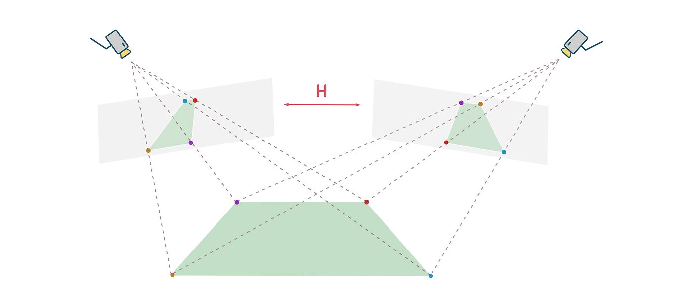
In this assignment, we learn to project the logo from an image to a sequence of video frames. Given a sequence of frames in a video and the corners in each frame that the logo should project onto, we can estimate the homography from the corresponding points. $$\lambda \mathbf{x} _{logo} = \mathbf{H} \mathbf{x} _{video}$$

$$ \lambda \begin{bmatrix} x\\ y\\ 1 \end{bmatrix} _{logo} = \begin{bmatrix} h _{11} & h _{12} & h _{13} \\ h _{21} & h _{22} & h _{23} \\h _{31} & h _{32} & 1 \end{bmatrix} \begin{bmatrix} x\\ y\\ 1 \end{bmatrix} _{video} $$

Since the homography matrix has eight DoF and each corresponding point imposes two constraints, we need at least 4 points to estimate the homography.

Pose Estimation

Similar to the 2D homography, we can estimate the camera pose by computing the homography from the image to the 3D world coordinate.

$$ \begin{bmatrix} u\\ v\\ w \end{bmatrix} \sim K\begin{bmatrix} r_1 & r_2 & r_3 & T \end{bmatrix} \begin{bmatrix} X\\ Y\\ Z\\ W \end{bmatrix} $$

If we assume all the points in the world coordinate lie in the ground plane $Z=0$, the transformation becomes

$$ \begin{bmatrix} u\\ v\\ w \end{bmatrix} \sim K\begin{bmatrix} r_1 & r_2 & T \end{bmatrix} \begin{bmatrix} X\\ Y\\ W \end{bmatrix} $$.

Then given the intrinsic matrix $K$ and the corresponding coordinates in each frame, we can compute the camera pose by solving for $\mathbf{R}$ and $\mathbf{T}$.

In this assignment, the goal is to project a 3D cube on an AprilTag in the video with the corner coordinates in the first frame given. Then we can apply the Kanade–Lucas–Tomasi tracker to get the corner coordinates in each consecutive frame and solve for the homography.

After we solve the homograph, to ensure the rotation matrix in the first two columns is orthogonal, we need to use Singular Value Decomposition to get the estimation of $\mathbf{R}$ and $\mathbf{T}$.

Multi-view Geometry

Moving on to the task of estimating the camera pose from a collection of images, similar to human vision, when we possess images captured from the same scene, we can deduce the camera’s position relative to the scene. This process is facilitated by a fundamental concept known as Epipolar Geometry, which provides a structured framework for understanding the geometric relationships between multiple cameras observing a common scene. Epipolar geometry plays an important role in computer vision and 3D reconstruction.

Epipolar Geometry

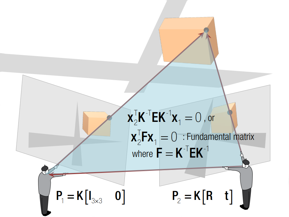
In the typical configuration of epipolar geometry, two cameras observe a common point $X$ in the scene. As shown in the following figure, the point is projected onto the image planes of the cameras, denoted as $P_1$ and $P_2$. The line connecting the two camera centers is known as the baseline. The plane defined by the two camera centers and X is called the epipolar plane. The points where the baseline intersects the two image planes are known as the epipoles. The lines where the intersection of the epipolar plane and the two image planes are known as the epipolar lines. If we select the point $P_1$ as the reference point, we can establish a relationship between $P_2$ and $P_1$ using a combination of translation and rotation matrices. Furthermore, we can denote the world point in the first and second camera’s view as $X_1$ and $X_2$ respectively.

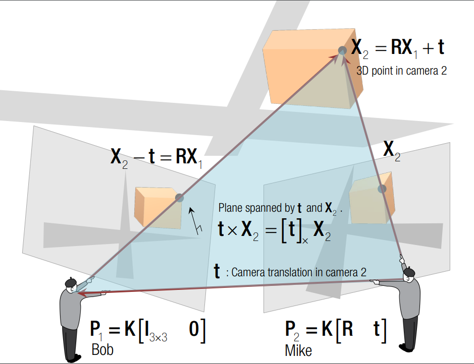
The constraint from the points $X_1$ and $X_2$ is shown in the following equation $$ X_2^T E X_1 = 0.$$

The matrix $E$ is called the Essential Matrix. The essential matrix encodes the rotation and translation between two points $X_1$ and $X_2$. Similarly, we have the constraint between the image point $x_1$ and $x_2$ as $$ x_2^TFx_1=0. $$

The matrix $F$ is called the Fundamental Matrix. It encodes the rotation and translation as well as the intrinsic parameters of the cameras. The fundamental matrix and essential matrix is related by $$ F = K^{-T}EK^{-1} .$$

Given two images for the same scene, we can use Scale-invariant feature transform (SIFT) to detect and describe local features of images.

The fundamental matrix has $8$ DoF, to estimate the fundamental matrix, we need at least 8 correspondence points. $$ \begin{bmatrix} u_i^2 & v_i^2 & 1 \end{bmatrix}\begin{bmatrix} f_{11} & f_{12} & f_{13} \\ f_{21} & f_{22} & f_{23} \\ f_{31} & f_{32} & f_{33} \end{bmatrix}\begin{bmatrix} u_i^1 \\ v_i^1 \\ 1 \end{bmatrix} = 0$$

After estimating the fundamental matrix, if we know the intrinsic parameter of the camera, we can estimate the essential matrix and recover the camera pose $R$ and $T$. The camera poses from the essential matrix do not uniquely define a world point $X$ in the homogeneous coordinate. To find the world point that corresponds to the point in the image, we need multiple sets of point measurements. Then we can reconstruct those rays, and try to find the intersection of the rays into the 3D space. This procedure is called Triangulation.

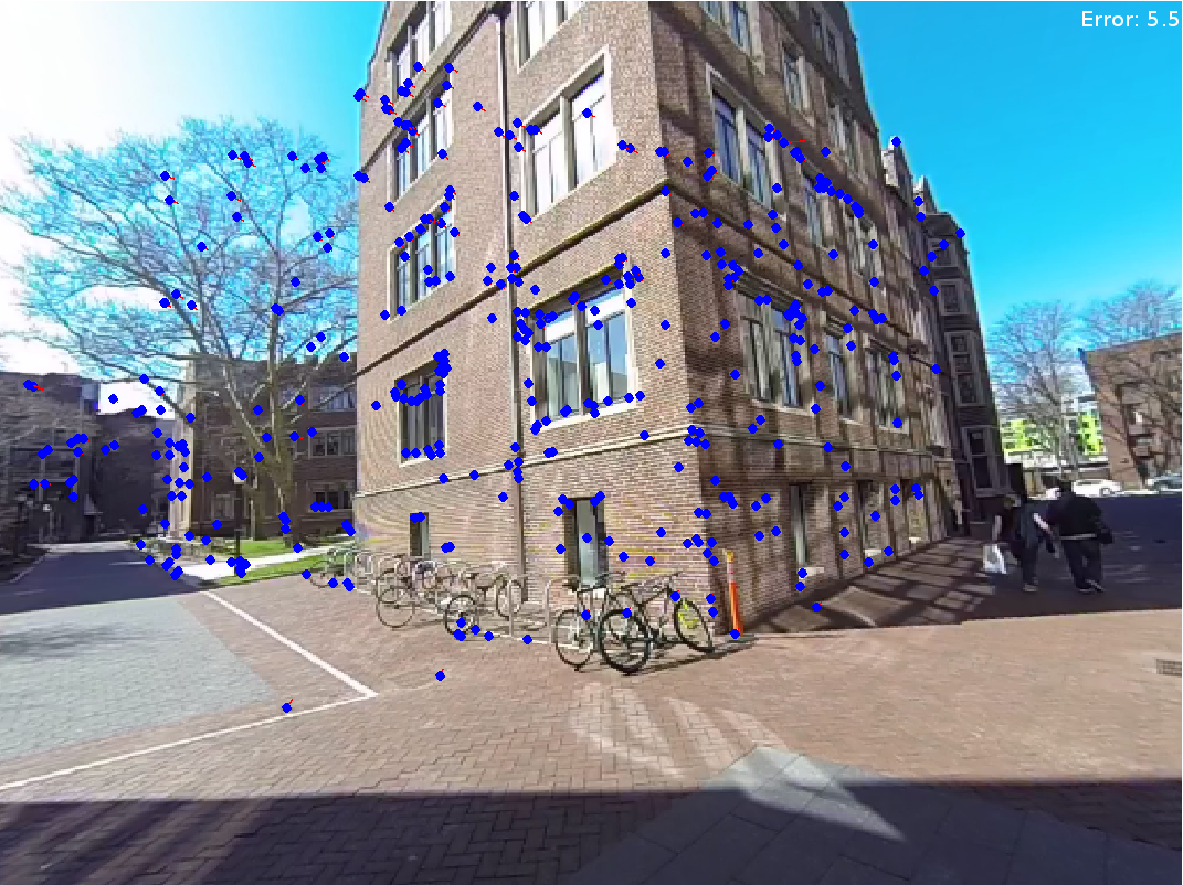
Structure from Motion

In this assignment, we implemented key elements of structure from motion (SfM) except for bundle adjustment. We are given three images of Levine Hall at the University of Pennsylvania, and correspondence points that are established by nearest neighbor search in SIFT local descriptors filtered by Random sample consensus (RANSAC) based on the fundamental matrix.

The following figures show the corresponding points in the images and the error in reprojection points.

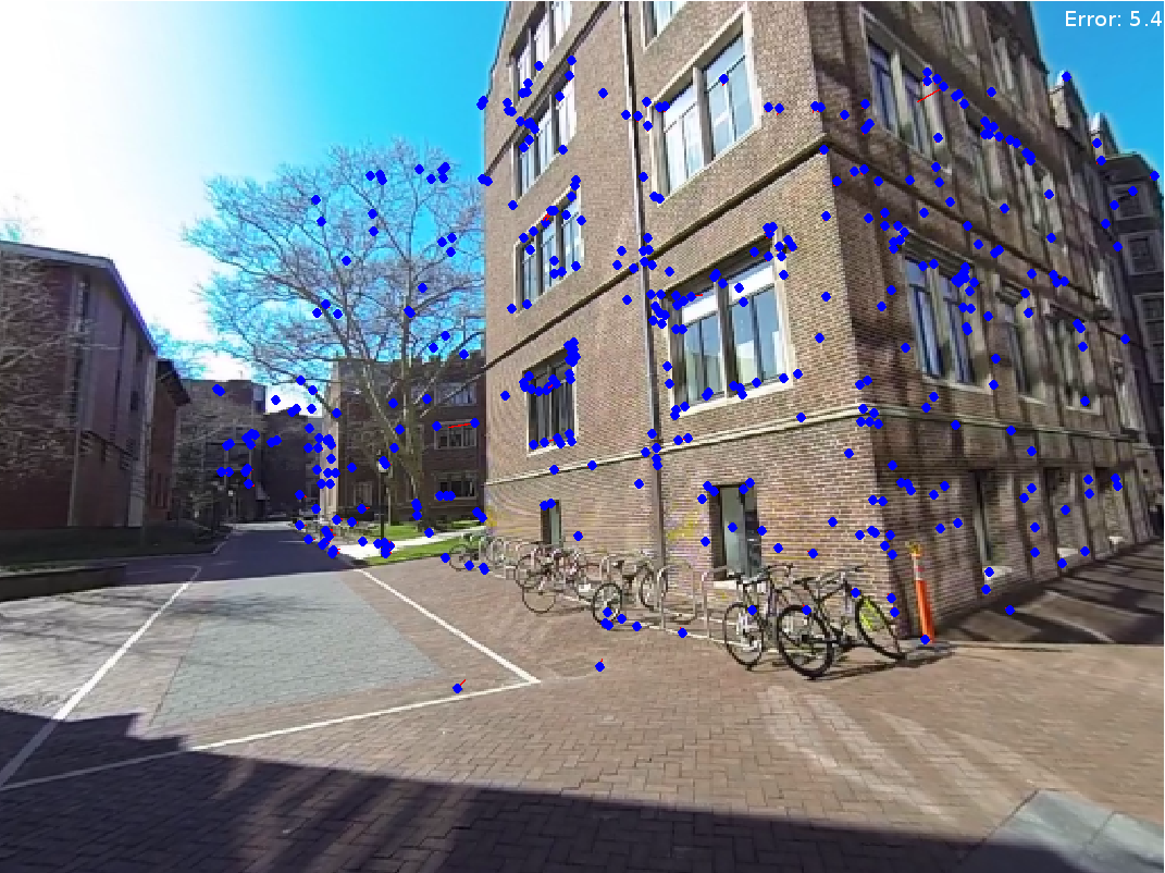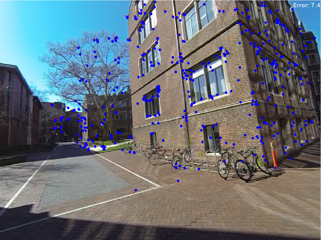The camera pose and reconstructed 3D points are shown in the following figure.

(Images and codes are from Robotics: Perception.)